
本文内容
原理简介
使用千人基因组项目数据与PLINK进行PCA
绘图
参考
1.原理简介
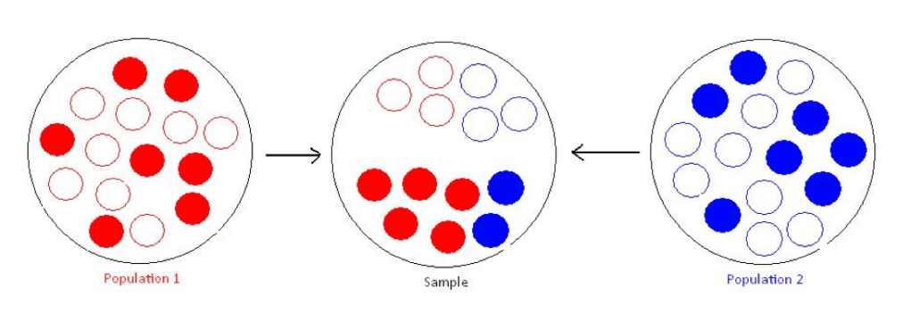
主成分分析(Principal Components Analysis, PCA)是一种常用的数据降维方法,在群体遗传学中被广泛用于识别并调整样本的群体分层问题。群体分层会导致GWAS研究中的虚假关联,考虑一个case-control研究,如下图所示,红色的群体在整体样本中占了case的大多数,那么一些对疾病并没有影响,但在红蓝两群体之间等位基因频率相差很大的genetic marker,就有可能会造成虚假关联(spurious association)。
假设我们有N个样本,M个SNP的数据,其对应的矩阵记为G,Gij则为第i个样本的第j个SNP,取值范围为0, 0.5, 1 ,对应有0,1,2个参考等位基因。
首先对G进行标准化(减去均值后除以标准差),得到的标准化后N x M矩阵记为Z,
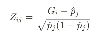
其中pj为第j个SNP的等位基因频率。
于是我们可以计算得到遗传关系矩阵GRM
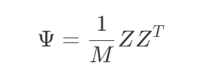
GRM中第i行第j列的项就表示个体i与个体j的遗传相似性的均值。
对GRM进行特征分解即可得到对应不同的群体结构特征的主成分PC。
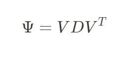
其中V是n个特征向量Vn组成的n x n 的矩阵,D则对应由n个特征值λn组成的向量。
这个n个特征值由大到小,λ1>λ2>…>λn, 特征值的大小与相对应特征向量所能解释方差成正比(也就是,第一主成分PC1能解释最多的方差,以此类推)。
主成分可以被视为反映 由于祖先不同而造成的样本遗传变异的连续方差轴。
对于某一主成分,有相似值的个体有着相似的对应祖先。
2 .下面介绍如何使用PLINK来进行PCA分析,并去除异常个体
本教程改编自: https://www.biostars.org/p/335605/
2.1软件与硬件要求
软件版本要求:
plink > v1.9
BCFtools (tested on v 1.3)
磁盘容量要求:
- downloaded data (VCF.gz and tab-indices), ~ 15.5 GB
- converted BCF files and their indices, ~14 GB
- binary PLINK files, ~53 GB
- pruned PLINK binary files, ~ <1 Gb
2.2 下载所用数据 (本教程数据主要来自1000 Genomes Phase III imputed genotypes)
2.3 下载对应每条染色体的vcf文件
prefix="ftp://ftp.1000genomes.ebi.ac.uk/vol1/ftp/release/20130502/ALL.chr" ;

suffix=".phase3_shapeit2_mvncall_integrated_v5b.20130502.genotypes.vcf.gz" ;

for chr in {1..22}; do
    wget "${prefix}""${chr}""${suffix}" "${prefix}""${chr}""${suffix}".tbi ;
done
2.4 下载 1000 Genomes Phase III 的 ped文件,包含了个体性别,群体等基本信息
wget ftp://ftp.1000genomes.ebi.ac.uk/vol1/ftp/technical/working/20130606_sample_info/20130606_g1k.ped ;
2.5 下载参考基因组 (GRCh37 / hg19)注:不同版本的区别详见
wget ftp://ftp.1000genomes.ebi.ac.uk/vol1/ftp/technical/reference/human_g1k_v37.fasta.gz ;
wget ftp://ftp.1000genomes.ebi.ac.uk/vol1/ftp/technical/reference/human_g1k_v37.fasta.fai ;

gunzip human_g1k_v37.fasta.gz ;
2.6 将 1000 genome 的文件转化成 BCF 格式,这一步需要对原始vcf文件进行预处理:
- 将multi-allelic calls分离(很多位点有3个及以上等位基因),并依据参考基因组标准化indels (详见:Variant Normalization 变异的标准化)
- 将ID filed设为 CHROM:POS:REF:ALT 这个格式,确保唯一性 (文件中有很多重复的rsID,却指向不同的位置)
x ID -I +'%CHROM:%POS:%REF:%ALT'先抹掉现有ID,然后重新将ID设为 CHROM:POS:REF:ALT - 去掉重复的变异
for chr in {1..22}; do
    bcftools norm -m-any --check-ref w -f human_g1k_v37.fasta \
      ALL.chr"${chr}".phase3_shapeit2_mvncall_integrated_v5b.20130502.genotypes.vcf.gz | \
      bcftools annotate -x ID -I +'%CHROM:%POS:%REF:%ALT' | \
        bcftools norm -Ob --rm-dup both \
          > ALL.chr"${chr}".phase3_shapeit2_mvncall_integrated_v5b.20130502.genotypes.bcf ;

    bcftools index ALL.chr"${chr}".phase3_shapeit2_mvncall_integrated_v5b.20130502.genotypes.bcf ;
done
2.7 将BCF转化成PLINK格式
for chr in {1..22}; do
    plink --noweb \
      --bcf ALL.chr"${chr}".phase3_shapeit2_mvncall_integrated_v5b.20130502.genotypes.bcf \
      --keep-allele-order \
      --vcf-idspace-to _ \
      --const-fid \
      --allow-extra-chr 0 \
      --split-x b37 no-fail \
      --make-bed \
      --out ALL.chr"${chr}".phase3_shapeit2_mvncall_integrated_v5b.20130502.genotypes ;
done
2.8 对每条染色体 Prune variants
mkdir Pruned ;

for chr in {1..22}; do
    plink --noweb \
      --bfile ALL.chr"${chr}".phase3_shapeit2_mvncall_integrated_v5b.20130502.genotypes \
      --maf 0.10 --indep 50 5 1.5 \
      --out Pruned/ALL.chr"${chr}".phase3_shapeit2_mvncall_integrated_v5b.20130502.genotypes ;

    plink --noweb \
      --bfile ALL.chr"${chr}".phase3_shapeit2_mvncall_integrated_v5b.20130502.genotypes \
      --extract Pruned/ALL.chr"${chr}".phase3_shapeit2_mvncall_integrated_v5b.20130502.genotypes.prune.in \
      --make-bed \
      --out Pruned/ALL.chr"${chr}".phase3_shapeit2_mvncall_integrated_v5b.20130502.genotypes ;
done
2.9 准备一个索引文件
find . -name "*.bim" | grep -e "Pruned" > ForMerge.list ;

sed -i 's/.bim//g' ForMerge.list ;
2.10 合并每条染色体的plink文件
如果有自己的文件需要合并,可以在这一步加进索引文件中
plink --merge-list ForMerge.list --out Merge ;
2.11 进行主成分分析 PCA
plink --bfile Merge --pca
3 . 绘图
需要之前下载好的ped文件,20130606_g1k.ped
以及群体的三个字母的编码对照表(如下所示,来自1000genomes.org的ftp)
#Populations

This file describes the population codes where assigned to samples collected for the 1000 Genomes project. These codes are used to organise the files in the data_collections' project data directories and can also be found in column 11 of many sequence index files.

There are also two tsv files, which contain the population codes and descriptions for both the sub and super populations that were used in phase 3 of the 1000 Genomes Project:

<ftp://ftp.1000genomes.ebi.ac.uk/vol1/ftp/phase3/20131219.populations.tsv>
<ftp://ftp.1000genomes.ebi.ac.uk/vol1/ftp/phase3/20131219.superpopulations.tsv>

###Populations and codes

         CHB	Han Chinese             Han Chinese in Beijing, China
         JPT	Japanese                Japanese in Tokyo, Japan
         CHS	Southern Han Chinese    Han Chinese South
         CDX	Dai Chinese             Chinese Dai in Xishuangbanna, China
         KHV	Kinh Vietnamese         Kinh in Ho Chi Minh City, Vietnam
         CHD	Denver Chinese          Chinese in Denver, Colorado (pilot 3 only)

         CEU	CEPH                    Utah residents (CEPH) with Northern and Western European ancestry
         TSI	Tuscan                  Toscani in Italia
         GBR	British                 British in England and Scotland
         FIN	Finnish                 Finnish in Finland
         IBS	Spanish                 Iberian populations in Spain

         YRI	Yoruba                  Yoruba in Ibadan, Nigeria
         LWK	Luhya                   Luhya in Webuye, Kenya
         GWD	Gambian                 Gambian in Western Division, The Gambia
         MSL	Mende                   Mende in Sierra Leone
         ESN	Esan                    Esan in Nigeria

         ASW	African-American SW     African Ancestry in Southwest US
         ACB	African-Caribbean       African Caribbean in Barbados
         MXL	Mexican-American        Mexican Ancestry in Los Angeles, California
         PUR	Puerto Rican            Puerto Rican in Puerto Rico
         CLM	Colombian               Colombian in Medellin, Colombia
         PEL	Peruvian                Peruvian in Lima, Peru

         GIH	Gujarati                Gujarati Indian in Houston, TX
         PJL	Punjabi                 Punjabi in Lahore, Pakistan
         BEB	Bengali                 Bengali in Bangladesh
         STU	Sri Lankan              Sri Lankan Tamil in the UK
         ITU	Indian                  Indian Telugu in the UK

Should you have any queries, please contact info@1000genomes.org.
下面演示用PYTHON进行绘图:
import pandas as pd
import numpy as np
import matplotlib.pyplot as plt
import seaborn as sns
#读取文件
pca = pd.read_csv("1000_all.eigenvec"," ",header=None)
ped = pd.read_csv("20130606_g1k.ped","\t")
#重命名pca文件的列
pca = pca.rename(columns=dict([(1,"Individual ID")]+[(x,"PC"+str(x-1)) for x in range(2,22)]))
#join两个数据表
pcaped=pca.join(ped,on="Individual ID",how="inner")
#给个体加上super population的标签
pcaped["Superpopulation"]="unknown"
pcaped.loc[pcaped["Population"].isin(["JPT","CHB","CDX","CHS","JPT","KHV","CHD"]),"Superpopulation"]="EAS"
pcaped.loc[pcaped["Population"].isin(["BEB","GIH","ITU","PJL","STU"]),"Superpopulation"]="SAS"
pcaped.loc[pcaped["Population"].isin(["CLM","MXL","PEL","PUR"]),"Superpopulation"]="AMR"
pcaped.loc[pcaped["Population"].isin(["CEU","FIN","GBR","IBS","TSI"]),"Superpopulation"]="EUR"
pcaped.loc[pcaped["Population"].isin(["ACB","ASW","ESN","GWD","LWK","MSL","YRI"]),"Superpopulation"]="AFR"
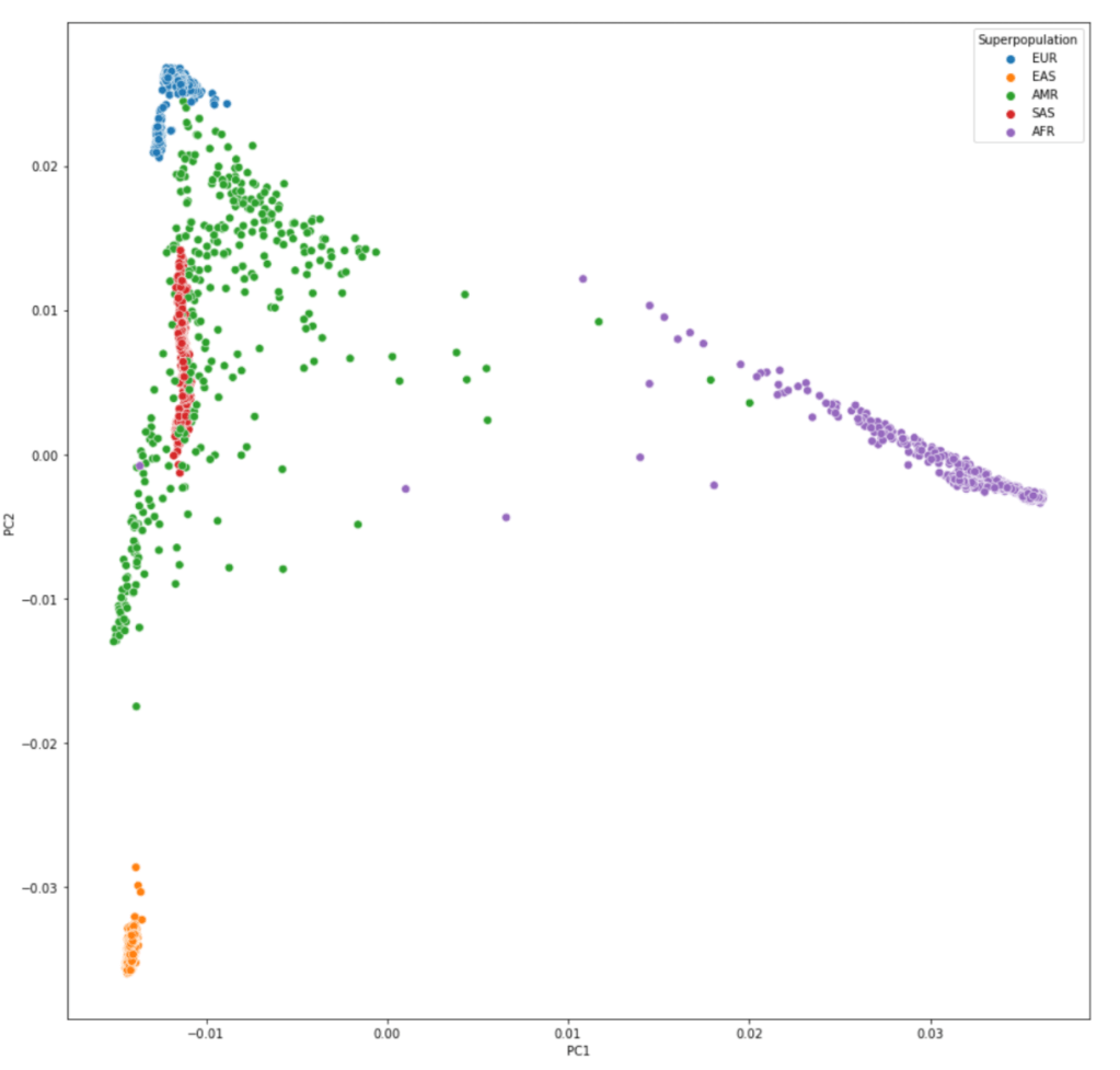
#绘制PC1与PC2的散点图,以Super population分不同颜色
plt.figure(figsize=(15,15))
sns.scatterplot(data=pcaped,x="PC1",y="PC2",hue="Superpopulation",s=50)
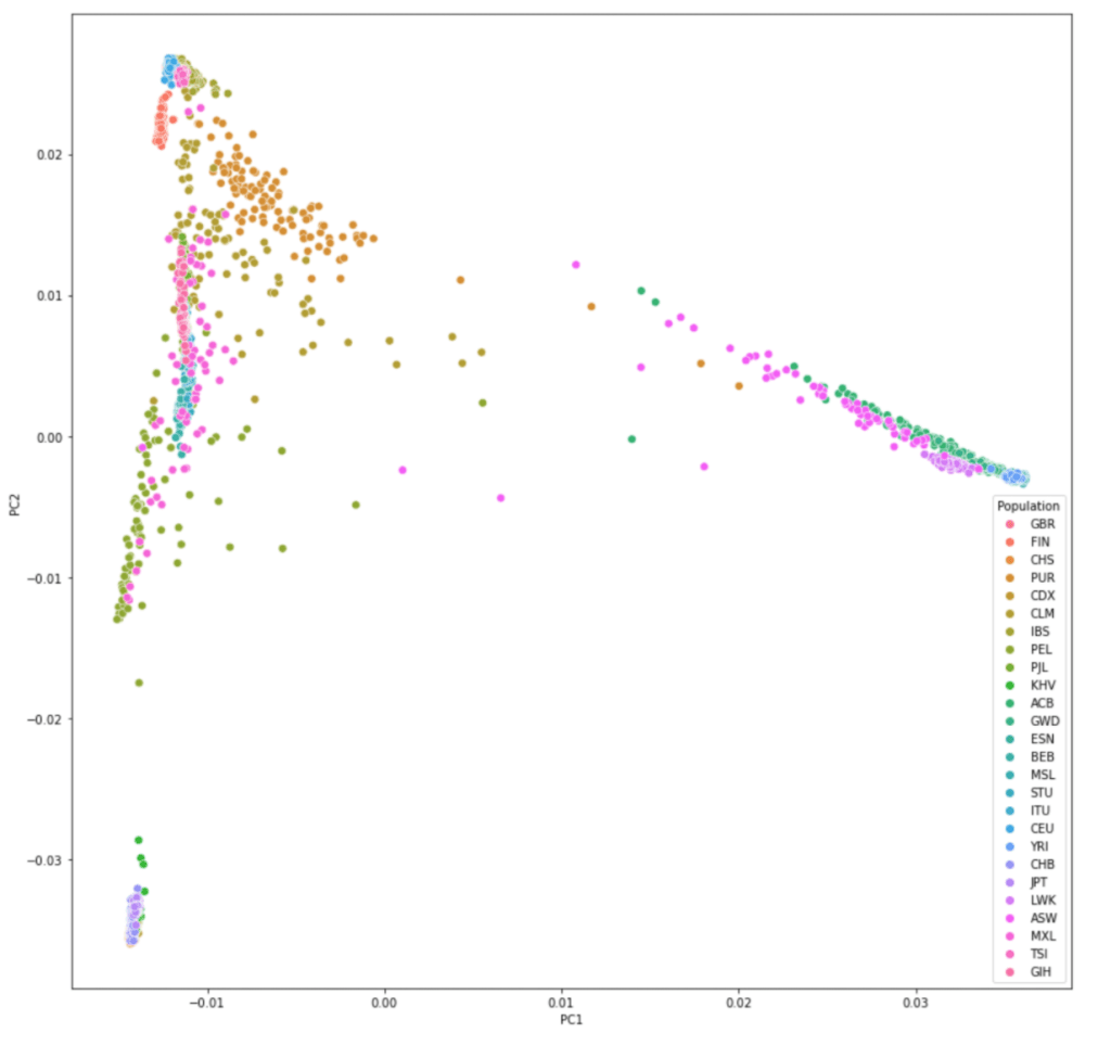
#绘制PC1与PC2的散点图,以Population分不同颜色
sns.scatterplot(data=pcaped,x="PC1",y="PC2",hue="Population",s=50)
参考:
https://www.cog-genomics.org/plink/1.9/strat
Price, A. L. et al. Principal components analysis corrects for stratification in genome-wide association studies. Nat. Genet. 38, 904–909 (2006).

