#CHROM	POS	ID	REF	ALT	QUAL	FILTER	INFO
1	10108	rs62651026	CAACCCT	C	46514.3	RF	AF_eas=0;AF_nfe=0;AF_fin=0.0227273
1	10109	rs376007522	AACCCT	A	89837.3	RF	AF_eas=0;AF_nfe=0.0512821;AF_fin=0.0588235
使用方法
输入选项
需要两个文件:一是gwas的sumstats,二是参考的vcf文件
Input files:
  --sumstats <file>     GWAS summary statistics file
  --vcf <file>          Reference VCF file. Use # as chromosome wildcard.
其中gwas sumstats还需要指定对应的列名:
Input column names:
  --chrom_col <str>     Chromosome column 染色体
  --pos_col <str>       Position column 碱基位置
  --effAl_col <str>     Effect allele column 效应等位
  --otherAl_col <str>   Other allele column 非效应等位
  --beta_col <str>      beta column
  --or_col <str>        Odds ratio column
  --or_col_lower <str>  Odds ratio lower CI column
  --or_col_upper <str>  Odds ratio upper CI column
  --eaf_col <str>       Effect allele frequency column
  --rsid_col <str>      rsID column in the summary stat file
Output files:
  --hm_sumstats <file>  Harmonised sumstat output file (use 'gz' extension to
                        gzip)
  --hm_statfile <file>  Statistics from harmonisation process output file.
                        Should only be used in conjunction with --hm_sumstats.
  --strand_counts <file>
                        Output file showing number of variants that are
                        forward/reverse/palindromic
其他选项
Other args:
  --only_chrom <str>    Only process this chromosome
  --in_sep <str>        Input file column separator (default: tab)
  --out_sep <str>       Output file column separator (default: tab)
  --na_rep_in <str>     How NA are represented in the input file (default: "")
  --na_rep_out <str>    How to represent NA values in output (default: "")
  --chrom_map <str> [<str> ...]
                        Map summary stat chromosome names, e.g. `--chrom_map
                        23=X 24=Y`
Harmonisation mode 模式选择:
可以选择以下四种模式:[infer|forward|reverse|drop]
对于 palindromic variants 的处理方式为:
(a) infer strand from effect-allele freq, 根据AF推测
(b) assume forward strand, 假设全部都为正链
(c) assume reverse strand, 假设全部为负链
(d) drop palindromic variants 舍弃所有palindromic variants
AF字段名与阈值
如果选择通过AF推测正负链(–palin_mode infer),那么还需要制定vcf文件中af的字段名与推测的阈值 –af_vcf_field <str> VCF info field containing alt allele freq (default:AF_NFE)
指定VCF文件中INFO里包含AF信息的字段
–infer_maf_threshold <float>Max MAF that will be used to infer palindrome strand (default: 0.42)
推测palindrome strand的最大MAF的阈值
使用例
如果输入的sumstats为以下格式:
CHROMOSOME POSITION MARKERNAME NEA EA EAF INFO N BETA SE P OR OR_95L OR_95U
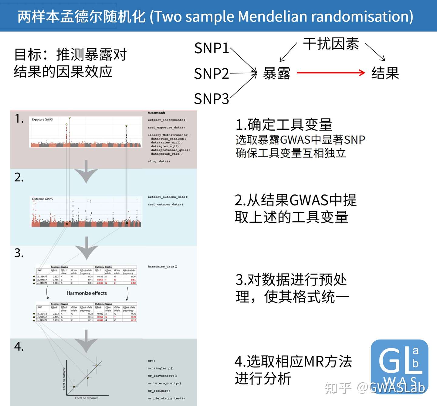
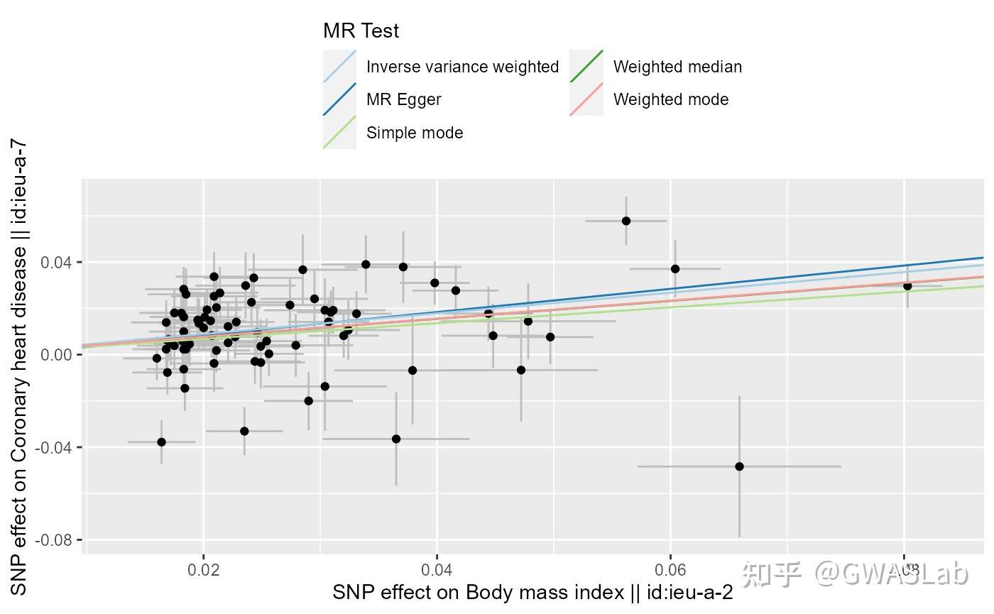
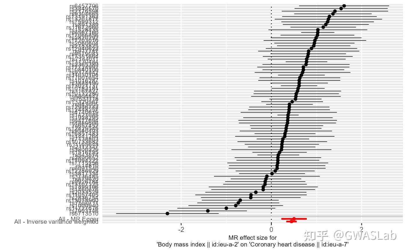
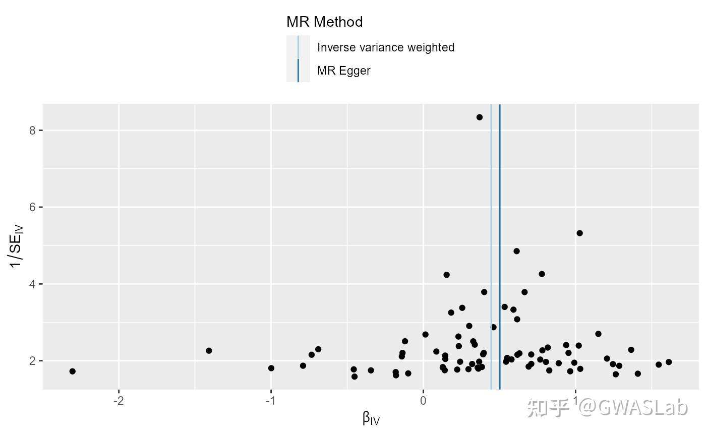
孟德尔随机化的原理可以参考G. Davey Smith and Ebrahim 2003; George Davey Smith and Hemani 2014, 统计方法可以参考Pierce and Burgess 2013; Bowden, Davey Smith, and Burgess 2015等。
bmi_exp_dat <- clump_data(bmi_exp_dat,clump_r2=0.01 ,pop = "EUR")
#> Please look at vignettes for options on running this locally if you need to run many instances of this command.
#> Clumping UVOe6Z, 30 variants, using EUR population reference
#> Removing 3 of 30 variants due to LD with other variants or absence from LD reference panel
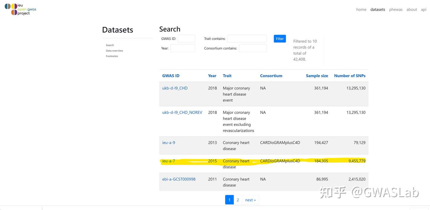
ao <- available_outcomes()
#> API: public: <http://gwas-api.mrcieu.ac.uk/>
head(ao)
#> # A tibble: 6 x 22
#>   id      trait     group_name  year consortium author sex   population    unit
#>   <chr>   <chr>     <chr>      <int> <chr>      <chr>  <chr> <chr>         <chr>
#> 1 ieu-b-~ Number o~ public      2021 MRC-IEU    Clare~ Male~ European      SD
#> 2 prot-a~ Leptin r~ public      2018 NA         Sun BB Male~ European      NA
#> 3 prot-a~ Adapter ~ public      2018 NA         Sun BB Male~ European      NA
#> 4 ukb-e-~ Impedanc~ public      2020 NA         Pan-U~ Male~ Greater Midd~ NA
#> 5 prot-a~ Dual spe~ public      2018 NA         Sun BB Male~ European      NA
#> 6 eqtl-a~ ENSG0000~ public      2018 NA         Vosa U Male~ European      NA
#> # ... with 13 more variables: sample_size <int>, nsnp <int>, build <chr>,
#> #   category <chr>, subcategory <chr>, ontology <chr>, note <chr>, mr <int>,
#> #   pmid <int>, priority <int>, ncase <int>, ncontrol <int>, sd <dbl>

## 使用grep1抓取目标表型
ao[grepl("heart disease", ao$trait), ]
#> # A tibble: 28 x 22
#>    id      trait       group_name  year consortium author sex   population unit
#>    <chr>   <chr>       <chr>      <int> <chr>      <chr>  <chr> <chr>      <chr>
#>  1 ieu-a-8 Coronary h~ public      2011 CARDIoGRAM Schun~ Male~ European   log ~
#>  2 finn-a~ Valvular h~ public      2020 NA         NA     Male~ European   NA
#>  3 finn-a~ Other or i~ public      2020 NA         NA     Male~ European   NA
#>  4 ukb-b-~ Diagnoses ~ public      2018 MRC-IEU    Ben E~ Male~ European   SD
#>  5 ukb-a-~ Diagnoses ~ public      2017 Neale Lab  Neale  Male~ European   SD
#>  6 ukb-e-~ I25 Chroni~ public      2020 NA         Pan-U~ Male~ South Asi~ NA
#>  7 ukb-b-~ Diagnoses ~ public      2018 MRC-IEU    Ben E~ Male~ European   SD
#>  8 finn-a~ Ischemic h~ public      2020 NA         NA     Male~ European   NA
#>  9 finn-a~ Major coro~ public      2020 NA         NA     Male~ European   NA
#> 10 finn-a~ Other hear~ public      2020 NA         NA     Male~ European   NA
#> # ... with 18 more rows, and 13 more variables: sample_size <int>, nsnp <int>,
#> #   build <chr>, category <chr>, subcategory <chr>, ontology <chr>, note <chr>,
#> #   mr <int>, pmid <int>, priority <int>, ncase <int>, ncontrol <int>, sd <dbl>
Hemani G, Tilling K, Davey Smith G (2017) Orienting the causal relationship between imprecisely measured traits using GWAS summary data. PLOS Genetics 13(11): e1007081. https://doi.org/10.1371/journal.pgen.1007081
Hemani G, Zheng J, Elsworth B, Wade KH, Baird D, Haberland V, Laurin C, Burgess S, Bowden J, Langdon R, Tan VY, Yarmolinsky J, Shihab HA, Timpson NJ, Evans DM, Relton C, Martin RM, Davey Smith G, Gaunt TR, Haycock PC, The MR-Base Collaboration. The MR-Base platform supports systematic causal inference across the human phenome. eLife 2018;7:e34408. doi: 10.7554/eLife.34408
Inouye, Michael, et al. “Genomic risk prediction of coronary artery disease in 480,000 adults: implications for primary prevention.” Journal of the American College of Cardiology 72.16 (2018): 1883-1893.
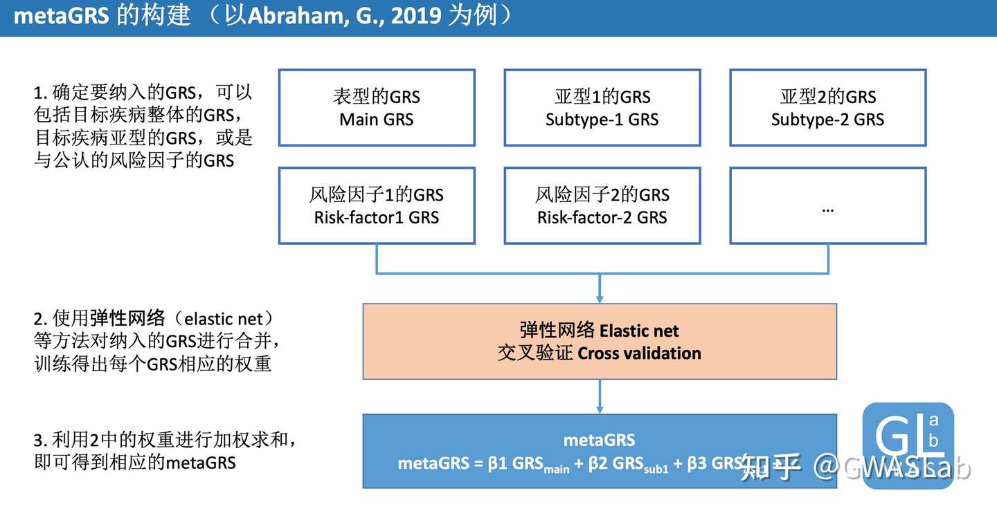
Abraham, G., Malik, R., Yonova-Doing, E. et al. Genomic risk score offers predictive performance comparable to clinical risk factors for ischaemic stroke. Nat Commun10, 5819 (2019). https://doi.org/10.1038/s41467-019-13848-1
Friedman, Jerome, Trevor Hastie, and Rob Tibshirani. “glmnet: Lasso and elastic-net regularized generalized linear models.” R package version 1.4 (2009): 1-24.
head -n 20 tutorial_results_1.1NS.log
2021/10/31/10:43:32 PM
<><><<>><><><><><><><><><><><><><><><><><><><><><><><><><><><><><><><><><><>
<>
<> MTAG: Multi-trait Analysis of GWAS
<> Version: 1.0.8
<> (C) 2017 Omeed Maghzian, Raymond Walters, and Patrick Turley
<> Harvard University Department of Economics / Broad Institute of MIT and Harvard
<> GNU General Public License v3
<><><<>><><><><><><><><><><><><><><><><><><><><><><><><><><><><><><><><><><>
<> Note:  It is recommended to run your own QC on the input before using this program.
<> Software-related correspondence: maghzian@nber.org
<> All other correspondence: paturley@broadinstitute.org
<><><<>><><><><><><><><><><><><><><><><><><><><><><><><><><><><><><><><><><>

Calling ./mtag.py \
--stream-stdout  \
--n-min 0.0 \
--sumstats 1_OA2016_hm3samp_NEUR.txt,1_OA2016_hm3samp_SWB.txt \
--out ./tutorial_results_1.1NS
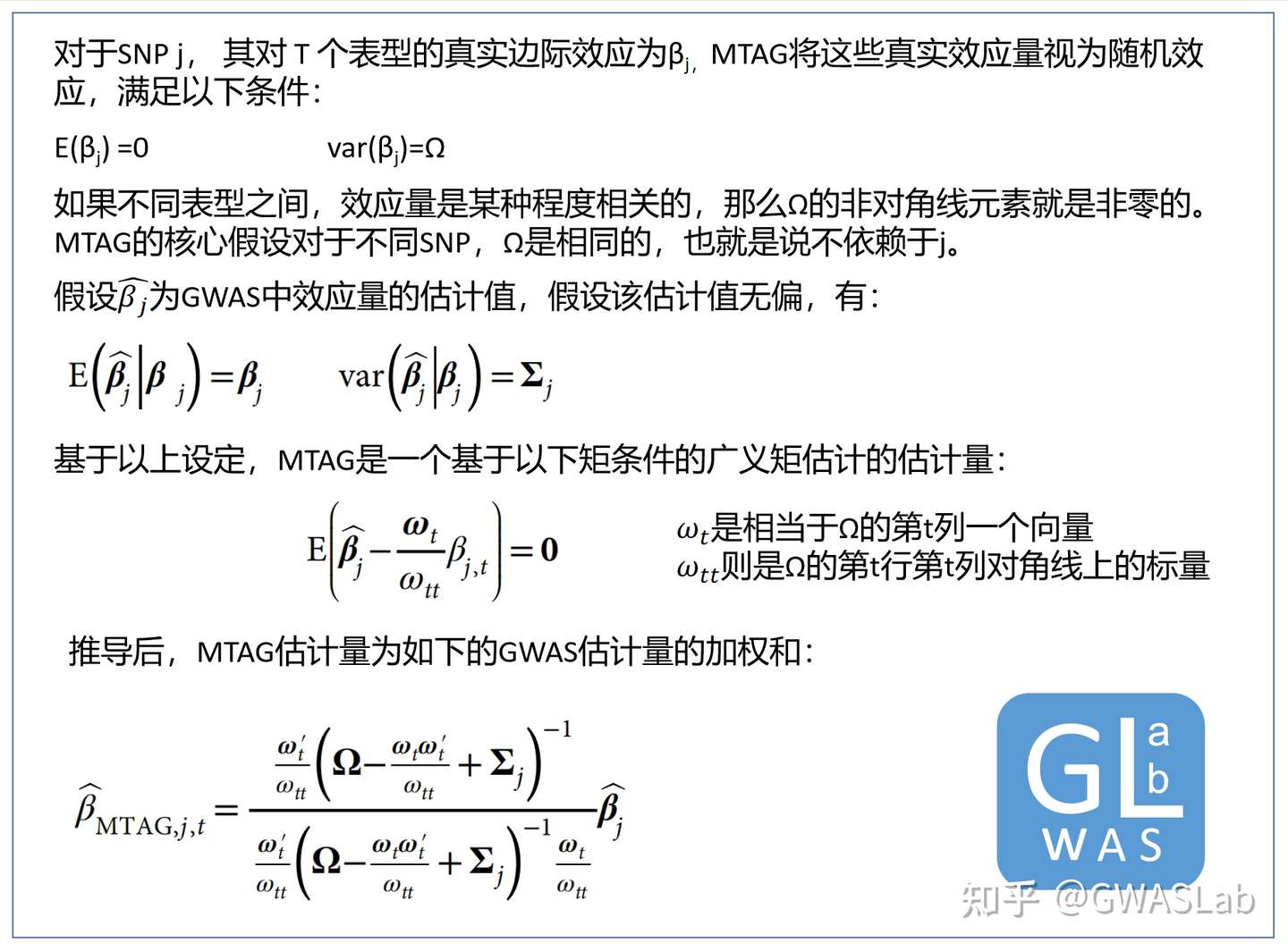
MTAG效应量估计值文件(trait_1):
head tutorial_results_1.1NS_trait_1.txt
SNP	CHR	BP	A1	A2	Z	N	FRQ	mtag_beta	mtag_se	mtag_z	mtag_pval
rs2736372	8	11106041	T	C	-7.7161416126199995	111111.11111099999	0.4179	-0.032488048690724455	0.004191057650619415	-7.751754186899077	9.063170638233748e-15
rs2060465	8	11162609	T	C	7.69444599845	62500.0	0.6194	0.038971244976047835	0.005364284755639267	7.264947099439278	3.731842884367329e-13
rs10096421	8	10831868	T	G	-7.561098219	111111.11111099999	0.4646	-0.0306226260844897350.004144573386350028	-7.388607518772383	1.483744201034853e-13
rs2409722	8	11039816	T	G	-7.382616018080001	111111.11111099999	0.4627	-0.032187004733709536	0.004145724613962613	-7.763903233057294	8.235474166666265e-15
rs11991118	8	10939273	T	G	7.32202915636	111111.11111099999	0.5056	0.030603923980300953 0.004134432028802615	7.402207550419989	1.339389362466671e-13
rs2736371	8	11105529	A	G	-7.32009158327	62500.0	0.3806	-0.03759068256663257	0.005364284755639268	-7.007585219467501	2.42466338629309e-12
rs2736313	8	11086942	T	C	-7.24228035161	111111.11111099999	0.4646	-0.03068115211425502 0.004144573386350028	-7.402728641577938	1.3341420385130596e-13
rs876954	8	8310923	A	G	-7.15791677597	62500.0	0.4813	-0.03422779585744538	0.005212736369758894 -6.566185862767606	5.162037825451834e-11
rs1533059	8	8684953	A	G	-7.074128564239999	62500.0	0.4478	-0.035027431607855014	0.00523771146606734	-6.687545091932079	2.269452965596589e-11
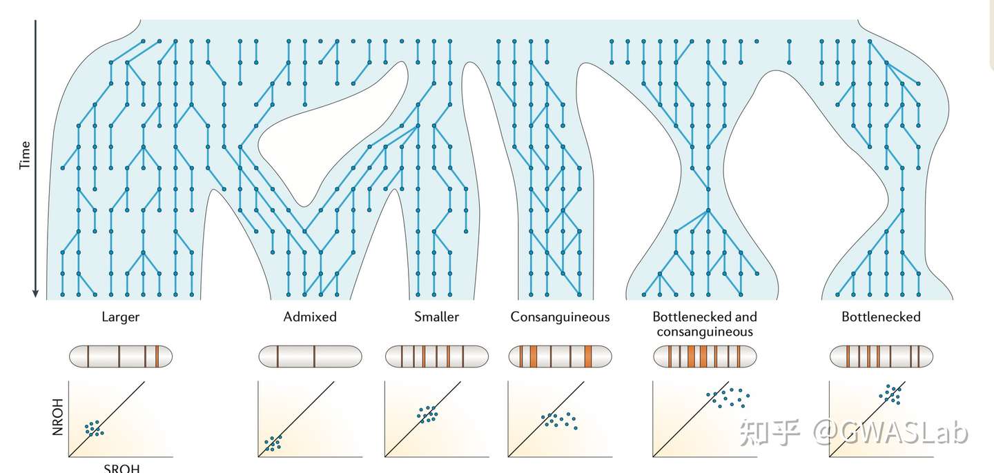
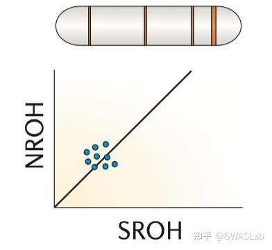
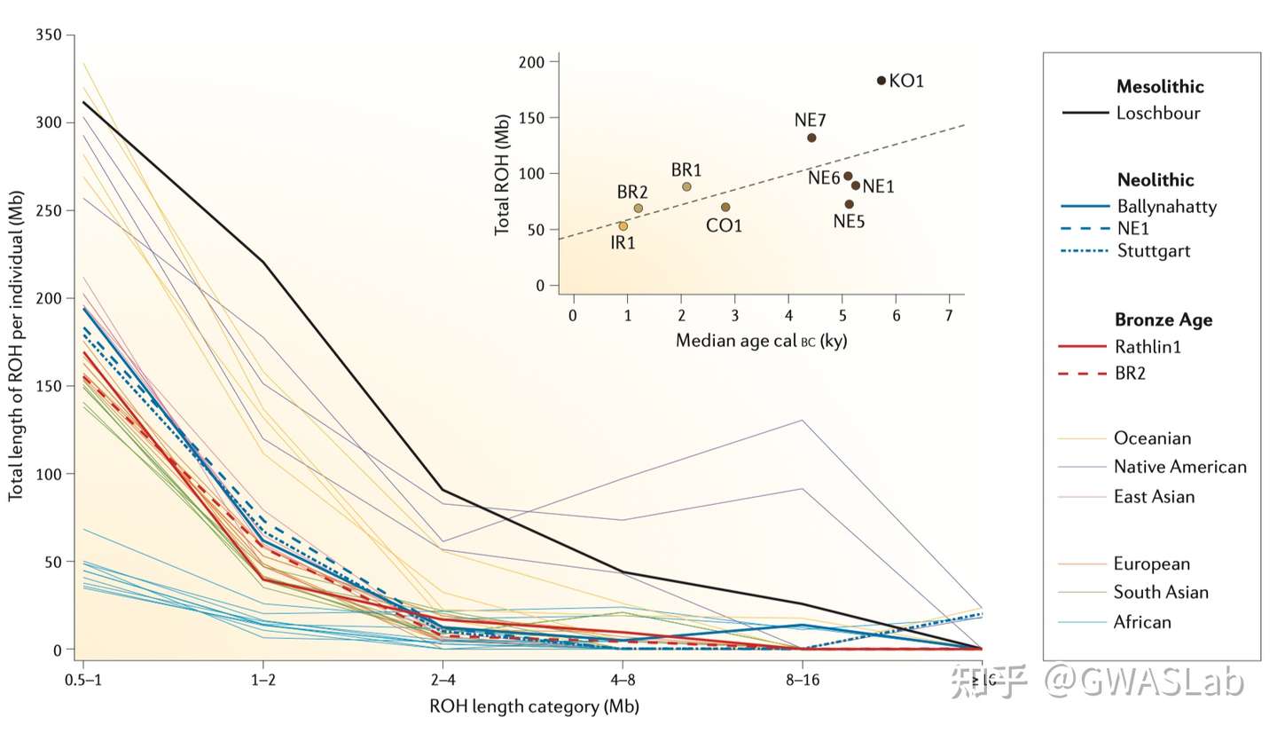
对于个体,其基因组上的一段区域内所有位点均为纯合的区域,被称为一段纯合性片段 (Runs of homozygosity,ROH). ROH的出现通常是由于个体来自父母双方的单倍体型是相同的,而这个单倍体型又是从过去某个时间点的共同祖先继承而来。ROH的概念不依赖于已知的家系,也不需要一个基线群体。但实际操作中,ROH通常规定有一个基于可用基因型密度的最小的长度,以判别是因为IBD而产生的ROH,或仅仅是概率偶然。
Ceballos, F. C., Joshi, P. K., Clark, D. W., Ramsay, M. & Wilson, J. F. Runs of homozygosity: windows into population history and trait architecture. Nat. Rev. Genet. 2018 194 19, 220–234 (2018).https://www.nature.com/articles/nrg.2017.109
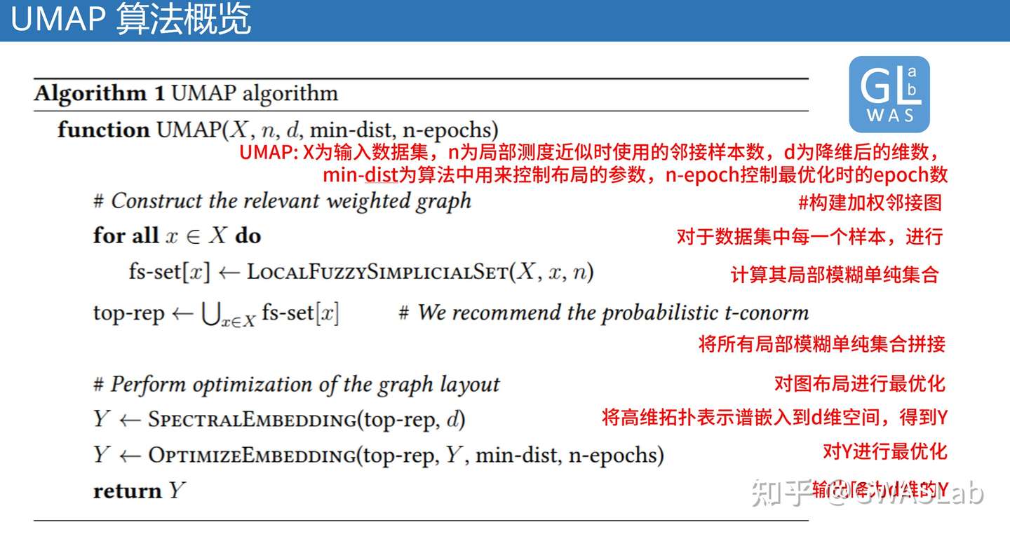
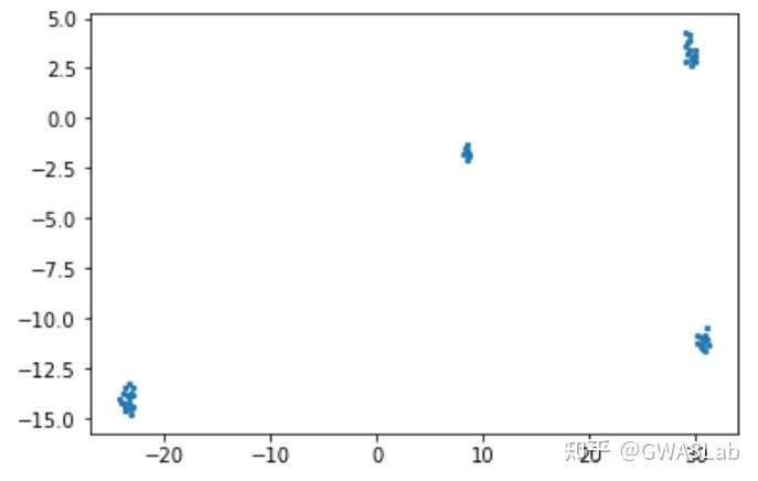
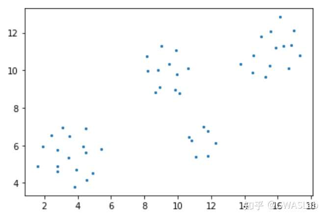
UMAP(uniform manifold approximation and projection)是近年来新出现的一种相对灵活的非线性降维算法,目前在统计遗传学等领域也有了较为广泛的应用。
UMAP的理论基础基于流形理论(manifold theory)与拓扑分析,
主要基于以下假设:
存在一个数据均一分布的流形。
这个目标流形是局部相连的。
该算法的主要目标是保存此流形的拓扑结构。
总体来看,UMAP利用了局部流形近似,并拼接模糊单纯集合表示(local fuzzy simplicial set representation),以构建高维数据的拓扑表示。在给定低维数据时,UMAP会采取相似的手法构建一个等价的拓扑表示。最后UMAP会对低维空间中数据表示的布局进行最优化,以最小化高维和低维两种拓扑表示之间的交叉熵(cross-entropy)。
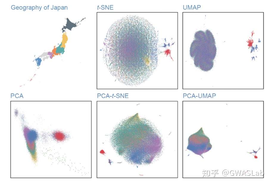
Sakaue, S., Hirata, J., Kanai, M. et al. Dimensionality reduction reveals fine-scale structure in the Japanese population with consequences for polygenic risk prediction. Nat Commun 11, 1569 (2020). https://doi.org/10.1038/s41467-020-15194-z
可以参考:Sakaue, S., Hirata, J., Kanai, M. et al. Dimensionality reduction reveals fine-scale structure in the Japanese population with consequences for polygenic risk prediction. Nat Commun 11, 1569
该文章对日本人群结构做了分析,并对比了各种降维方法的结果,强烈推荐。
参考
McInnes, L, Healy, J, UMAP: Uniform Manifold Approximation and Projection for Dimension Reduction, ArXiv e-prints 1802.03426, 2018
Sakaue, S., Hirata, J., Kanai, M. et al. Dimensionality reduction reveals fine-scale structure in the Japanese population with consequences for polygenic risk prediction. Nat Commun 11, 1569
Diaz-Papkovich, A., Anderson-Trocmé, L. & Gravel, S. A review of UMAP in population genetics. J. Hum. Genet. 66, 85–91 (2021).
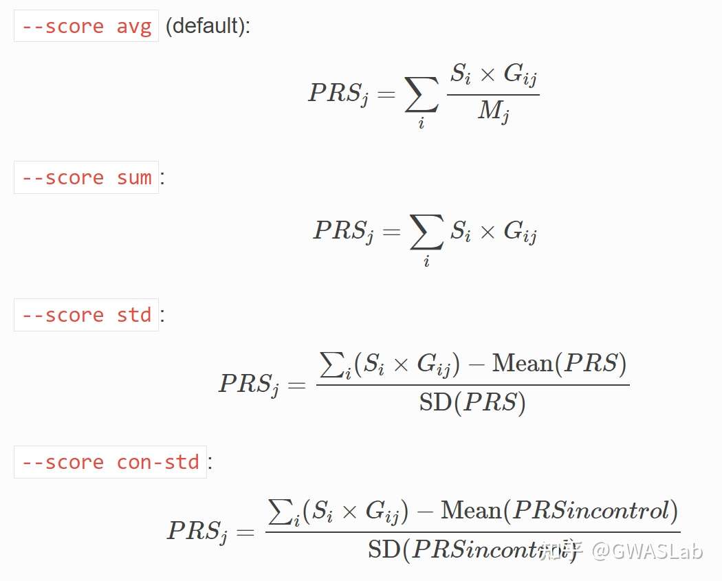
prsice	PRSice_xxx	指定PRSice二进制文件路径
base	        Height.QC.gz	 输入的base的GWAS summary statistic target
EUR.QC	指定target的plink文件名的前缀
binary-target	F	指定表型是否为二进制表型,F为否
pheno	EUR.height	提供表型文件
cov	EUR.covariate	        提供协变量文件
base-maf	MAF:0.01	使用base文件中MAF列来过滤掉maf<0.01的变异
base-info	INFO:0.8	使用base文件中INFO列来过滤掉info<0.8的变异 stat
OR	base文件中包含效应量的列名
or	-	指定效应量的形式为OR
out	EUR	指定输出前缀为EUR
执行后log文件如下所示:
PRSice 2.3.3 (2020-08-05)
<https://github.com/choishingwan/PRSice>
(C) 2016-2020 Shing Wan (Sam) Choi and Paul F. O'Reilly
GNU General Public License v3
If you use PRSice in any published work, please cite:
Choi SW, O'Reilly PF.
PRSice-2: Polygenic Risk Score Software for Biobank-Scale Data.
GigaScience 8, no. 7 (July 1, 2019)
2021-09-06 12:47:56
PRSice_linux \
    --a1 A1 \
    --a2 A2 \
    --bar-levels 0.001,0.05,0.1,0.2,0.3,0.4,0.5,1 \
    --base Height.QC.gz \
    --base-info INFO:0.8 \
    --base-maf MAF:0.01 \
    --binary-target F \
    --bp BP \
    --chr CHR \
    --clump-kb 250kb \
    --clump-p 1.000000 \
    --clump-r2 0.100000 \
    --cov EUR.covariate \
    --interval 5e-05 \
    --lower 5e-08 \
    --num-auto 22 \
    --or  \
    --out EUR \
    --pheno EUR.height \
    --pvalue P \
    --seed 3490962723 \
    --snp SNP \
    --stat OR \
    --target EUR.QC \
    --thread 1 \
    --upper 0.5

Initializing Genotype file: EUR.QC (bed)

Start processing Height.QC
==================================================

Base file: Height.QC.gz
GZ file detected. Header of file is:
CHR	BP	SNP	A1	A2	N	SE	P	OR	INFO	MAF

Reading 100.00%
499617 variant(s) observed in base file, with:
499617 total variant(s) included from base file

Loading Genotype info from target
==================================================

483 people (232 male(s), 251 female(s)) observed
483 founder(s) included

489805 variant(s) included

Phenotype file: EUR.height
Column Name of Sample ID: FID+IID
Note: If the phenotype file does not contain a header, the
column name will be displayed as the Sample ID which is
expected.

There are a total of 1 phenotype to process

Start performing clumping

Clumping Progress: 100.00%
Number of variant(s) after clumping : 193758

Processing the 1 th phenotype

Height is a continuous phenotype
11 sample(s) without phenotype
472 sample(s) with valid phenotype

Processing the covariate file: EUR.covariate
==============================

Include Covariates:
Name	Missing	Number of levels
Sex	0	-
PC1	0	-
PC2	0	-
PC3	0	-
PC4	0	-
PC5	0	-
PC6	0	-

After reading the covariate file, 472 sample(s) included in
the analysis

Start Processing
Processing 100.00%
There are 1 region(s) with p-value less than 1e-5. Please
note that these results are inflated due to the overfitting
inherent in finding the best-fit PRS (but it's still best
to find the best-fit PRS!).
You can use the --perm option (see manual) to calculate an
empirical P-value.

Begin plotting
Current Rscript version = 2.3.3
Plotting Bar Plot
Plotting the high resolution plot
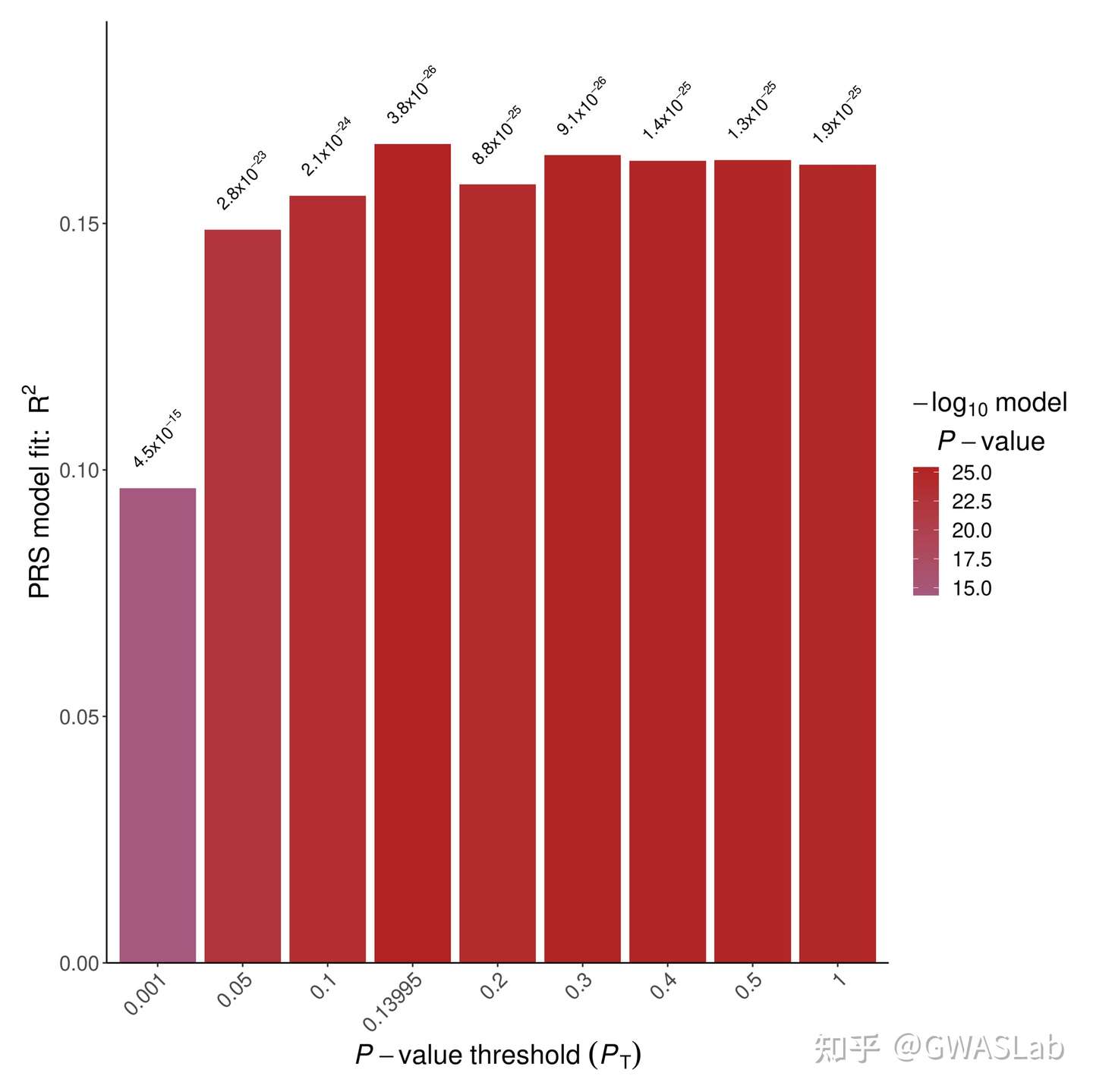
默认输出结果中有两张图,以及两个文本文件:
第一张为柱状图可以看到不同P值阈值下PRS模型R2的大小:
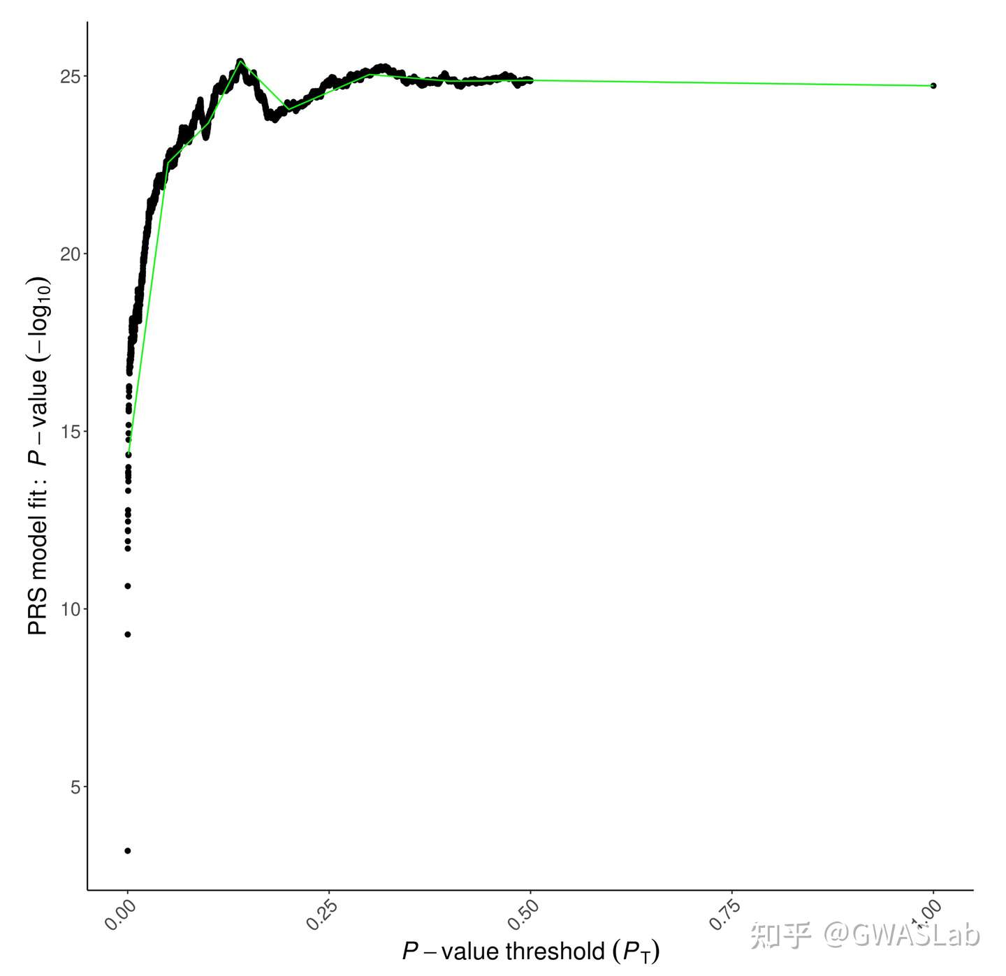
第二种则是高精度图,表示所有p值阈值的模型拟合:
第一个后缀为prsice的文本文件各个C+T参数的模型的结果:
head EUR.prsice
Pheno	Set	Threshold	R2	P	Coefficient	Standard.Error	Num_SNP
-	Base	5e-08	0.0192512	0.000644758	563.907	164.163	1999
-	Base	5.005e-05	0.0619554	5.24437e-10	3080.12	485.501	7615
-	Base	0.00010005	0.0713244	2.27942e-11	3816.99	557.044	9047
-	Base	0.00015005	0.0785205	2.00391e-12	4362.01	603.601	10014
-	Base	0.00020005	0.0799241	1.24411e-12	4666.13	639.344	10756
-	Base	0.00025005	0.0820088	6.11958e-13	4947.48	668.217	11365
-	Base	0.00030005	0.0818422	6.47686e-13	5146.63	695.905	11884
-	Base	0.00035005	0.0836689	3.47353e-13	5392.8	720.237	12373
-	Base	0.00040005	0.0849879	2.21299e-13	5589.41	739.972	12817