文章:Hingorani, A. D., Gratton, J., Finan, C., Schmidt, A. F., Patel, R., Sofat, R., … & Wald, N. J. (2023). Performance of polygenic risk scores in screening, prediction, and risk stratification: secondary analysis of data in the Polygenic Score Catalog. BMJ medicine, 2(1).
Hingorani等人的文章主要研究对象为PGS Catalog中已发表PGS的性能指标估计值(hazard ratio, odds ratio等), 并将其转化为临床检验常用的指标 DR5 (detection rate for a 5% false positive rate)进行二次分析。这篇文章得出了负面的结论,PRS在疾病筛查,预测以及风险分层等方面表现较差,对PRS的强调与其在健康体系中的实际效果不成正比。
(批判性参考)Hingorani, A. D., Gratton, J., Finan, C., Schmidt, A. F., Patel, R., Sofat, R., … & Wald, N. J. (2023). Performance of polygenic risk scores in screening, prediction, and risk stratification: secondary analysis of data in the Polygenic Score Catalog. BMJ medicine, 2(1). https://bmjmedicine.bmj.com/content/2/1/e000554
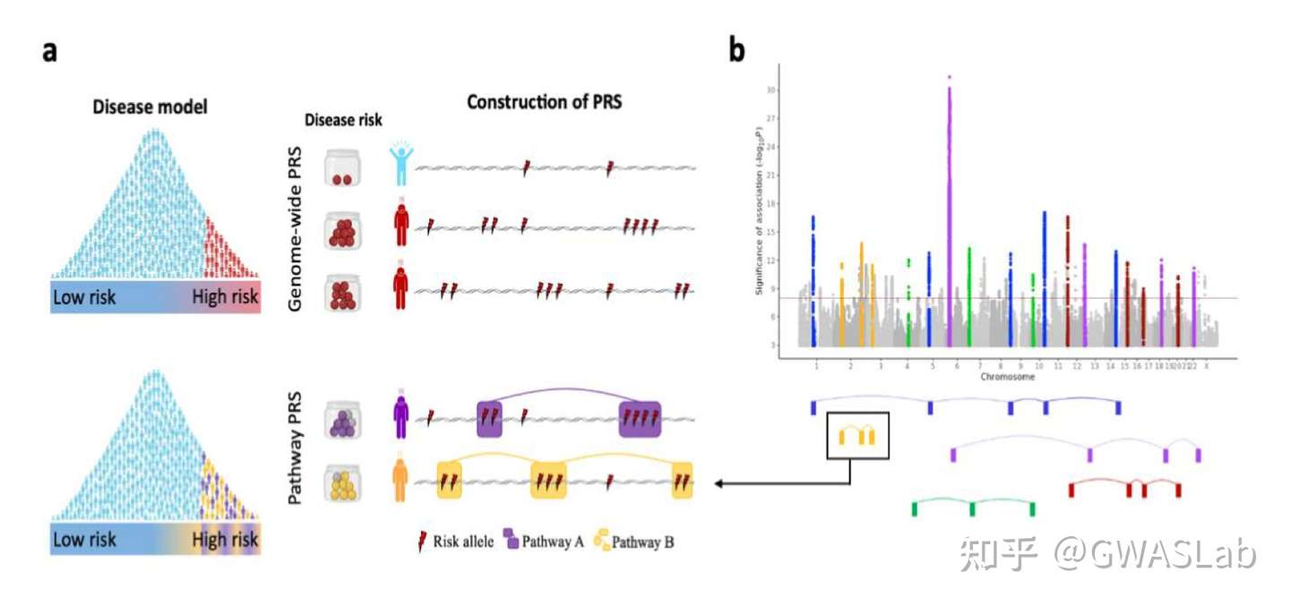
Lewis, C. M., & Vassos, E. (2020). Polygenic risk scores: from research tools to clinical instruments. Genome medicine, 12(1), 1-11.
*** 2 discovery populations detected ***
##### process chromosome 22 #####
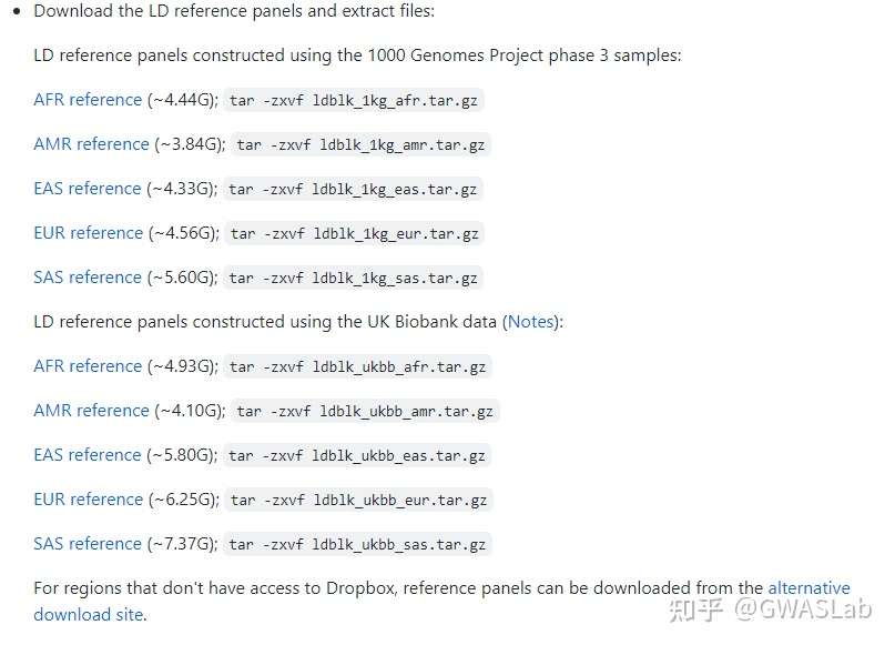
... parse reference file: /home/heyunye/tools/prscs/ldref/snpinfo_mult_1kg_hm3 ...
... 18944 SNPs on chromosome 22 read from /home/heyunye/tools/prscs/ldref/snpinfo_mult_1kg_hm3 ...
... parse bim file: /home/heyunye/tools/prscsx/PRScsx/test_data/test.bim ...
... 1000 SNPs on chromosome 22 read from /home/heyunye/tools/prscsx/PRScsx/test_data/test.bim ...
... parse EUR sumstats file: /home/heyunye/tools/prscsx/PRScsx/test_data/EUR_sumstats.txt ...
... 1000 SNPs read from /home/heyunye/tools/prscsx/PRScsx/test_data/EUR_sumstats.txt ...
... 1000 common SNPs in the EUR reference, EUR sumstats, and validation set ...
... parse EAS sumstats file: /home/heyunye/tools/prscsx/PRScsx/test_data/EAS_sumstats.txt ...
... 1000 SNPs read from /home/heyunye/tools/prscsx/PRScsx/test_data/EAS_sumstats.txt ...
... 901 common SNPs in the EAS reference, EAS sumstats, and validation set ...
... parse EUR reference LD on chromosome 22 ...
... parse EAS reference LD on chromosome 22 ...
... align reference LD on chromosome 22 across populations ...
... 1000 valid SNPs across populations ...
... MCMC ...
--- iter-100 ---
--- iter-200 ---
--- iter-300 ---
--- iter-400 ---
--- iter-500 ---
--- iter-600 ---
--- iter-700 ---
--- iter-800 ---
--- iter-900 ---
--- iter-1000 ---
--- iter-1100 ---
--- iter-1200 ---
--- iter-1300 ---
--- iter-1400 ---
--- iter-1500 ---
--- iter-1600 ---
--- iter-1700 ---
--- iter-1800 ---
--- iter-1900 ---
--- iter-2000 ---
... Done ...
输出为EUR以及EAS的PRS:
test_EAS_pst_eff_a1_b0.5_phi1e-02_chr22.txt
test_EUR_pst_eff_a1_b0.5_phi1e-02_chr22.txt
head test_EAS_pst_eff_a1_b0.5_phi1e-02_chr22.txt
22      rs9605903       17054720        C       T       8.694291e-04
22      rs5746647       17057138        G       T       -1.005430e-03
22      rs5747999       17075353        C       A       -2.499230e-04
22      rs2845380       17203103        A       G       6.037999e-04
22      rs2247281       17211075        G       A       4.780305e-04
22      rs2845346       17214252        C       T       7.767527e-04
22      rs2845347       17214669        C       T       1.671207e-03
22      rs1807512       17221495        C       T       -1.778397e-03
22      rs5748593       17227461        T       C       9.849030e-04
22      rs9606468       17273728        C       T       1.442600e-04
Ruan, Y., Lin, Y. F., Feng, Y. C. A., Chen, C. Y., Lam, M., Guo, Z., … & Ge, T. (2022). Improving polygenic prediction in ancestrally diverse populations. Nature Genetics, 54(5), 573-580.
Ge, T., Irvin, M. R., Patki, A., Srinivasasainagendra, V., Lin, Y. F., Tiwari, H. K., … & Karlson, E. W. (2022). Development and validation of a trans-ancestry polygenic risk score for type 2 diabetes in diverse populations. Genome medicine, 14(1), 1-16.
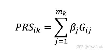
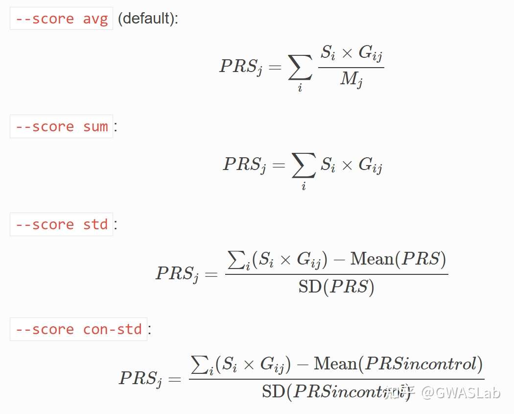
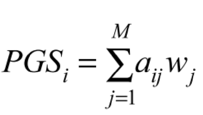
--score applies one or more linear scoring systems to each sample, and reports results to plink2.sscore. More precisely, if G is the full genotype/dosage matrix (rows = alleles, columns = samples) and a is a scoring-system vector with one coefficient per allele, --score computes the vector-matrix product aTG, and then divides by the number of variants when reporting score-averages.
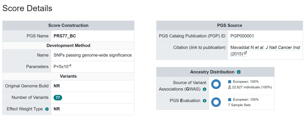
###PGS CATALOG SCORING FILE - see <https://www.pgscatalog.org/downloads/#dl_ftp_scoring> for additional information
#format_version=2.0
##POLYGENIC SCORE (PGS) INFORMATION
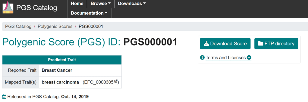
#pgs_id=PGS000001
#pgs_name=PRS77_BC
#trait_reported=Breast Cancer
#trait_mapped=breast carcinoma
#trait_efo=EFO_0000305
#weight_type=NR
#genome_build=NR
#variants_number=77
##SOURCE INFORMATION
#pgp_id=PGP000001
#citation=Mavaddat N et al. J Natl Cancer Inst (2015). doi:10.1093/jnci/djv036
rsID chr_name effect_allele other_allele effect_weight locus_name OR
rs78540526 11 T C 0.16220387987485377 CCND1 1.1761
...
Header	Column set	Contents
FID	maybefid, fid	Family ID
IID	(required)	Individual ID
SID	maybesid, sid	Source ID
PHENO1	pheno1	All-missing phenotype column, if none loaded
<Pheno name>, ...	pheno1, phenos	Phenotype value(s) (only first if just 'pheno1')
ALLELE_CT	nallele	Number of alleles across scored variants
DENOM	denom	Denominator used for score average
NAMED_ALLELE_DOSAGE_SUM	dosagesum	Sum of named allele dosages
<Score name>_AVG, ...	scoreavgs	Score averages
<Score name>_SUM, ...	scoresums	Score sums #分染色体时使用这一列求和
Samuel A. Lambert, Laurent Gil, Simon Jupp, Scott C. Ritchie, Yu Xu, Annalisa Buniello, Aoife McMahon, Gad Abraham, Michael Chapman, Helen Parkinson, John Danesh, Jacqueline A. L. MacArthur and Michael Inouye.
The Polygenic Score Catalog as an open database for reproducibility and systematic evaluation
Inouye, Michael, et al. “Genomic risk prediction of coronary artery disease in 480,000 adults: implications for primary prevention.” Journal of the American College of Cardiology 72.16 (2018): 1883-1893.
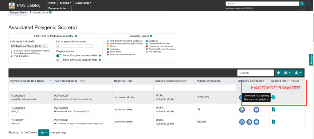
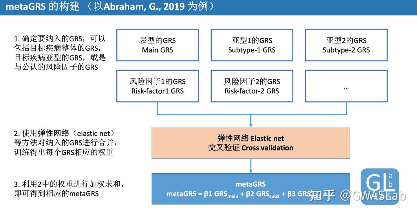
Abraham, G., Malik, R., Yonova-Doing, E. et al. Genomic risk score offers predictive performance comparable to clinical risk factors for ischaemic stroke. Nat Commun10, 5819 (2019). https://doi.org/10.1038/s41467-019-13848-1
Friedman, Jerome, Trevor Hastie, and Rob Tibshirani. “glmnet: Lasso and elastic-net regularized generalized linear models.” R package version 1.4 (2009): 1-24.
prsice	PRSice_xxx	指定PRSice二进制文件路径
base	        Height.QC.gz	 输入的base的GWAS summary statistic target
EUR.QC	指定target的plink文件名的前缀
binary-target	F	指定表型是否为二进制表型,F为否
pheno	EUR.height	提供表型文件
cov	EUR.covariate	        提供协变量文件
base-maf	MAF:0.01	使用base文件中MAF列来过滤掉maf<0.01的变异
base-info	INFO:0.8	使用base文件中INFO列来过滤掉info<0.8的变异 stat
OR	base文件中包含效应量的列名
or	-	指定效应量的形式为OR
out	EUR	指定输出前缀为EUR
执行后log文件如下所示:
PRSice 2.3.3 (2020-08-05)
<https://github.com/choishingwan/PRSice>
(C) 2016-2020 Shing Wan (Sam) Choi and Paul F. O'Reilly
GNU General Public License v3
If you use PRSice in any published work, please cite:
Choi SW, O'Reilly PF.
PRSice-2: Polygenic Risk Score Software for Biobank-Scale Data.
GigaScience 8, no. 7 (July 1, 2019)
2021-09-06 12:47:56
PRSice_linux \
    --a1 A1 \
    --a2 A2 \
    --bar-levels 0.001,0.05,0.1,0.2,0.3,0.4,0.5,1 \
    --base Height.QC.gz \
    --base-info INFO:0.8 \
    --base-maf MAF:0.01 \
    --binary-target F \
    --bp BP \
    --chr CHR \
    --clump-kb 250kb \
    --clump-p 1.000000 \
    --clump-r2 0.100000 \
    --cov EUR.covariate \
    --interval 5e-05 \
    --lower 5e-08 \
    --num-auto 22 \
    --or  \
    --out EUR \
    --pheno EUR.height \
    --pvalue P \
    --seed 3490962723 \
    --snp SNP \
    --stat OR \
    --target EUR.QC \
    --thread 1 \
    --upper 0.5

Initializing Genotype file: EUR.QC (bed)

Start processing Height.QC
==================================================

Base file: Height.QC.gz
GZ file detected. Header of file is:
CHR	BP	SNP	A1	A2	N	SE	P	OR	INFO	MAF

Reading 100.00%
499617 variant(s) observed in base file, with:
499617 total variant(s) included from base file

Loading Genotype info from target
==================================================

483 people (232 male(s), 251 female(s)) observed
483 founder(s) included

489805 variant(s) included

Phenotype file: EUR.height
Column Name of Sample ID: FID+IID
Note: If the phenotype file does not contain a header, the
column name will be displayed as the Sample ID which is
expected.

There are a total of 1 phenotype to process

Start performing clumping

Clumping Progress: 100.00%
Number of variant(s) after clumping : 193758

Processing the 1 th phenotype

Height is a continuous phenotype
11 sample(s) without phenotype
472 sample(s) with valid phenotype

Processing the covariate file: EUR.covariate
==============================

Include Covariates:
Name	Missing	Number of levels
Sex	0	-
PC1	0	-
PC2	0	-
PC3	0	-
PC4	0	-
PC5	0	-
PC6	0	-

After reading the covariate file, 472 sample(s) included in
the analysis

Start Processing
Processing 100.00%
There are 1 region(s) with p-value less than 1e-5. Please
note that these results are inflated due to the overfitting
inherent in finding the best-fit PRS (but it's still best
to find the best-fit PRS!).
You can use the --perm option (see manual) to calculate an
empirical P-value.

Begin plotting
Current Rscript version = 2.3.3
Plotting Bar Plot
Plotting the high resolution plot
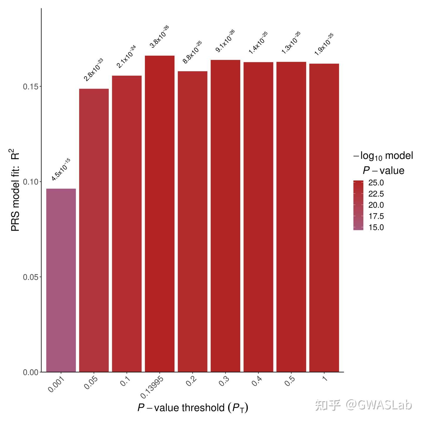
默认输出结果中有两张图,以及两个文本文件:
第一张为柱状图可以看到不同P值阈值下PRS模型R2的大小:
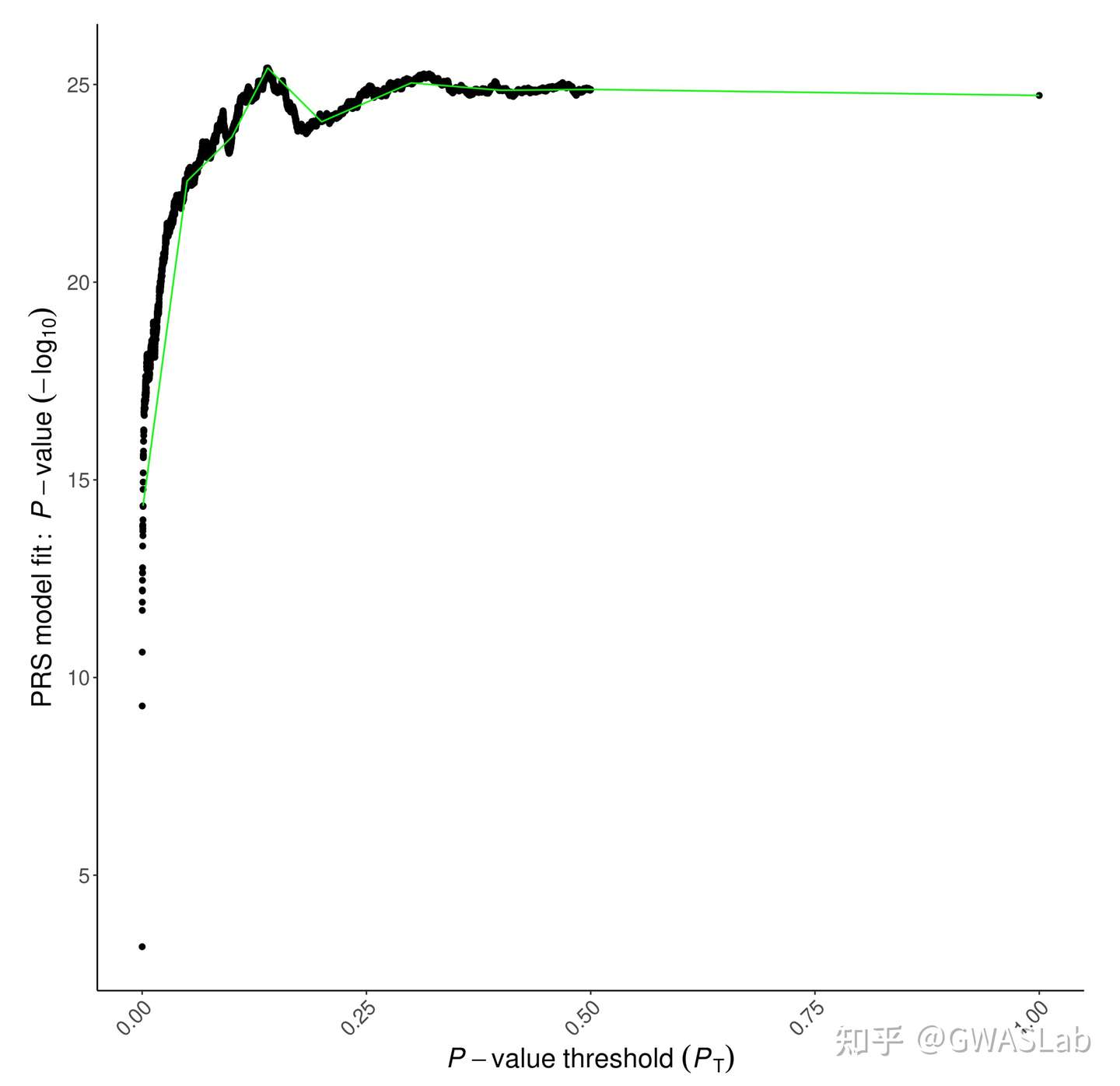
第二种则是高精度图,表示所有p值阈值的模型拟合:
第一个后缀为prsice的文本文件各个C+T参数的模型的结果:
head EUR.prsice
Pheno	Set	Threshold	R2	P	Coefficient	Standard.Error	Num_SNP
-	Base	5e-08	0.0192512	0.000644758	563.907	164.163	1999
-	Base	5.005e-05	0.0619554	5.24437e-10	3080.12	485.501	7615
-	Base	0.00010005	0.0713244	2.27942e-11	3816.99	557.044	9047
-	Base	0.00015005	0.0785205	2.00391e-12	4362.01	603.601	10014
-	Base	0.00020005	0.0799241	1.24411e-12	4666.13	639.344	10756
-	Base	0.00025005	0.0820088	6.11958e-13	4947.48	668.217	11365
-	Base	0.00030005	0.0818422	6.47686e-13	5146.63	695.905	11884
-	Base	0.00035005	0.0836689	3.47353e-13	5392.8	720.237	12373
-	Base	0.00040005	0.0849879	2.21299e-13	5589.41	739.972	12817
head Height.QC
CHR	BP	SNP	A1	A2	N	SE	P	OR	INFO	MAF
1	756604	rs3131962	A	G	388028	0.00301666	0.483171	0.997886915712650.890557941364774	0.369389592764921
1	768448	rs12562034	A	G	388028	0.00329472	0.834808	1.000687316093530.895893511351165	0.336845754096289
1	779322	rs4040617	G	A	388028	0.00303344	0.42897	0.997603556067569	0.897508290615237	0.377368010940814
1	801536	rs79373928	G	T	388028	0.00841324	0.808999	1.002035699227930.908962856432993	0.483212245374095
1	808631	rs11240779	G	A	388028	0.00242821	0.590265	1.001308325111540.893212523690488	0.450409558999587
1	809876	rs57181708	G	A	388028	0.00336785	0.71475	1.00123165786833	0.923557624081969	0.499743932656759
1	835499	rs4422948	G	A	388028	0.0023758	0.710884	0.999119752645200.906437735120596	0.481016005816168
1	838555	rs4970383	A	C	388028	0.00235773	0.150993	0.996619945289750.907716506801574	0.327164029672754
1	840753	rs4970382	C	T	388028	0.00207377	0.199967	0.997345678956140.914602590137255	0.498936220426316
可以利用简单的R脚本进行转换,在这里我们在文件的最后一列后添加转换后的beta
dat <- read.table(gzfile("Height.QC.gz"), header=T)
dat$BETA <- log(dat$OR)
write.table(dat, "Height.QC.Transformed", quote=F, row.names=F)
q() # exit R
将OR转换成beta后
head Height.QC.Transformed
CHR BP SNP A1 A2 N SE P OR INFO MAF BETA
1 756604 rs3131962 A G 388028 0.00301666 0.483171 0.997886915712657 0.890557941364774 0.369389592764921 -0.00211532000000048
1 768448 rs12562034 A G 388028 0.00329472 0.834808 1.00068731609353 0.895893511351165 0.336845754096289 0.000687079999998082
1 779322 rs4040617 G A 388028 0.00303344 0.42897 0.997603556067569 0.897508290615237 0.377368010940814 -0.00239932000000021
1 801536 rs79373928 G T 388028 0.00841324 0.808999 1.00203569922793 0.908962856432993 0.483212245374095 0.00203362999999797
1 808631 rs11240779 G A 388028 0.00242821 0.590265 1.00130832511154 0.893212523690488 0.450409558999587 0.00130747000000259
1 809876 rs57181708 G A 388028 0.00336785 0.71475 1.00123165786833 0.923557624081969 0.499743932656759 0.00123090000000354
1 835499 rs4422948 G A 388028 0.0023758 0.710884 0.999119752645202 0.906437735120596 0.481016005816168 -0.000880634999999921
1 838555 rs4970383 A C 388028 0.00235773 0.150993 0.996619945289758 0.907716506801574 0.327164029672754 -0.0033857799999997
1 840753 rs4970382 C T 388028 0.00207377 0.199967 0.99734567895614 0.914602590137255 0.498936220426316 -0.00265785000000019
head EUR.clumped
CHR    F         SNP         BP        P    TOTAL   NSIG    S05    S01   S001  S0001    SP2
   6    1   rs3134762   31210866  4.52e-165      180     20      0      0      0    160 rs2523898(1),rs13210132(1),rs28732080(1),rs28732081(1),rs28732082(1),rs2517552(1),rs2517546(1),rs2844647(1),rs2517537(1),rs2844645(1),rs2523857(1),rs2517527(1),rs3131788(1),rs3132564(1),rs3130955(1),rs3130544(1),rs2535296(1),rs2517448(1),rs6457327(1),rs28732096(1),rs2233956(1),rs1265048(1),rs3130985(1),rs13201757(1),rs6909321(1),rs3130557(1),rs17196961(1),rs9501055(1),rs13200022(1),rs3130573(1),rs28732101(1),rs1265095(1),rs2233940(1),rs130079(1),rs746647(1),rs2240064(1),rs3131012(1)...
p.threshold <- c(0.001,0.05,0.1,0.2,0.3,0.4,0.5)
# Read in the phenotype file
phenotype <- read.table("EUR.height", header=T)
# Read in the PCs
pcs <- read.table("EUR.eigenvec", header=F)
# The default output from plink does not include a header
# To make things simple, we will add the appropriate headers
# (1:6 because there are 6 PCs)
colnames(pcs) <- c("FID", "IID", paste0("PC",1:6))
# Read in the covariates (here, it is sex)
covariate <- read.table("EUR.cov", header=T)
# Now merge the files
pheno <- merge(merge(phenotype, covariate, by=c("FID", "IID")), pcs, by=c("FID","IID"))
# We can then calculate the null model (model with PRS) using a linear regression
# (as height is quantitative)
null.model <- lm(Height~., data=pheno[,!colnames(pheno)%in%c("FID","IID")])
# And the R2 of the null model is
null.r2 <- summary(null.model)$r.squared
prs.result <- NULL
for(i in p.threshold){
    # Go through each p-value threshold
    prs <- read.table(paste0("EUR.",i,".profile"), header=T)
    # Merge the prs with the phenotype matrix
    # We only want the FID, IID and PRS from the PRS file, therefore we only select the
    # relevant columns
    pheno.prs <- merge(pheno, prs[,c("FID","IID", "SCORE")], by=c("FID", "IID"))
    # Now perform a linear regression on Height with PRS and the covariates
    # ignoring the FID and IID from our model
    model <- lm(Height~., data=pheno.prs[,!colnames(pheno.prs)%in%c("FID","IID")])
    # model R2 is obtained as
    model.r2 <- summary(model)$r.squared
    # R2 of PRS is simply calculated as the model R2 minus the null R2
    prs.r2 <- model.r2-null.r2
    # We can also obtain the coeffcient and p-value of association of PRS as follow
    prs.coef <- summary(model)$coeff["SCORE",]
    prs.beta <- as.numeric(prs.coef[1])
    prs.se <- as.numeric(prs.coef[2])
    prs.p <- as.numeric(prs.coef[4])
    # We can then store the results
    prs.result <- rbind(prs.result, data.frame(Threshold=i, R2=prs.r2, P=prs.p, BETA=prs.beta,SE=prs.se))
}
# Best result is:
prs.result[which.max(prs.result$R2),]
q() # exit R
执行后就可以看到本次PRS计算中,最优的阈值为0.3
Rscript bestfit.R
  Threshold        R2            P     BETA       SE
5       0.3 0.1638468 1.025827e-25 47343.32 4248.152
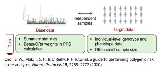
Choi, S. W., Mak, T. S. H. & O’Reilly, P. F. Tutorial: a guide to performing polygenic risk score analyses. Nature Protocols 15, 2759–2772 (2020).
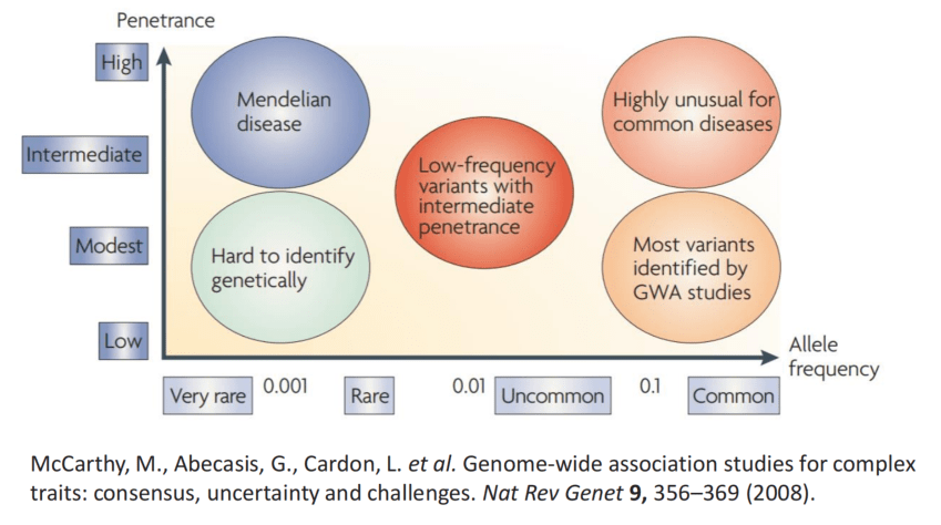
McCarthy, M., Abecasis, G., Cardon, L. et al. Genome-wide association studies for complex traits: consensus, uncertainty and challenges. Nat Rev Genet 9, 356–369 (2008).
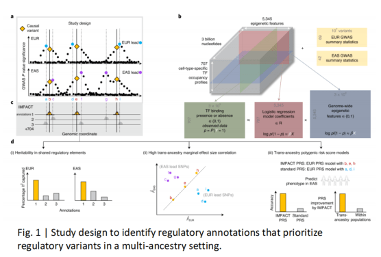
Amariuta, T. et al. Improving the trans-ancestry portability of polygenic risk scores by prioritizing variants in predicted cell-typespecific regulatory elements. Nature Genetics 52, 1346–1354 (2020).