09 孟德尔随机化 Mendelian randomization – GWASLab

TwoSampleMR简介
TwoSampleMR简要教程
1. 方法概览
2. 读取暴露GWAS数据，选取工具变量
3. 读取结局GWAS数据，提取对应工具变量
4. 对数据进行预处理，使其效应等位与效应量保持统一
5. MR分析与可视化
  1. MR分析
  2. 敏感性分析
  3. 散点图
  4. 森林图
  5. 漏斗图
参考

TwoSampleMR简介

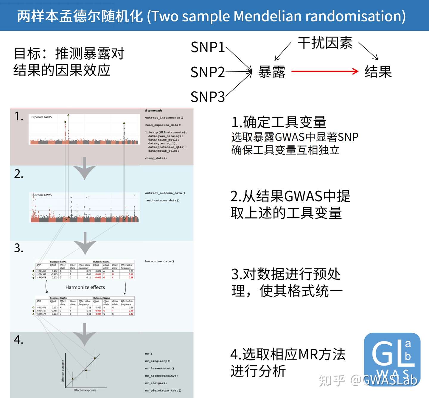
两样本孟德尔随机化（Two sample Mendelian randomisation，2SMR）是使用GWAS概括性数据估计暴露对结果的因果效应的一种方法。尽管孟德尔随机化在概念上相对直观简单，但实际操作却相对繁琐，有很多细节需要注意。TwoSampleMR就是一款致力于简化MR分析的R包，其整合了以下的分析步骤：

数据管理与统一
因果推断的常规统计学分析
接入了GWAS概括性数据的数据库，使分析更为便捷

孟德尔随机化的原理可以参考G. Davey Smith and Ebrahim 2003; George Davey Smith and Hemani 2014，统计方法可以参考Pierce and Burgess 2013; Bowden, Davey Smith, and Burgess 2015等。

TwoSampleMR简要教程

本文仅对TwoSampleMR使用方法进行介绍。基础概念概念可以参考：GWASLab：孟德尔随机化系列之一：基础概念 Mendelian randomization I

下载（注：本文所用语言均为R）

TwoSampleMR官网： https://mrcieu.github.io/TwoSampleMR/

TwoSampleMR是一个R包，可以通过以下代码在R中直接安装

install.packages("remotes")
remotes::install_github("MRCIEU/TwoSampleMR")

0 方法概览

MR分析的主要步骤如下：

读取暴露因素GWAS数据
选取合适的工具变量（如有必要，需要进行clumping）
读取结局GWAS数据，提取上述的工具变量的SNP
对暴露因素与结局的GWAS数据进行预处理，使其格式统一
采用选中的MR方法进行分析
将结果可视化
1. 散点图
2. 森林图
3. 漏斗图

1 读取暴露GWAS数据，选取工具变量

1.1 读取数据

对于暴露因素的GWAS数据，TwoSampleMR需要一个工具变量的data frame，每行对应一个SNP，至少需要4列，分别为：

SNP – rs ID
beta – The effect size. If the trait is binary then log(OR) should be used
se – The standard error of the effect size
effect_allele – The allele of the SNP which has the effect marked in beta

其他可能有助于MR预处理或分析的列包括

other_allele – The non-effect allele
eaf – The effect allele frequency
Phenotype – The name of the phenotype for which the SNP has an effect

你也可以提供额外的信息（可选，对于分析非必须）

chr – Physical position of variant (chromosome)
position – Physical position of variant (position)
samplesize – Sample size for estimating the effect size
ncase – Number of cases
ncontrol – Number of controls
pval – The P-value for the SNP’s association with the exposure
units – The units in which the effects are presented
gene – The gene or other annotation for the the SNP

本教程将从本地文本文件中读取暴露GWAS数据：

本文使用的暴露因素的GWAS数据的前5行如下所示：

rsid,effect,SE,a1,a2,a1_freq,p-value,Units,Gene,n
rs10767664,0.19,0.030612245,A,T,0.78,5.00E-26,kg/m2,BDNF,225238
rs13078807,0.1,0.020408163,G,A,0.2,4.00E-11,kg/m2,CADM2,221431
rs1514175,0.07,0.020408163,A,G,0.43,8.00E-14,kg/m2,TNNI3K,207641
rs1558902,0.39,0.020408163,A,T,0.42,5.00E-120,kg/m2,FTO,222476

该示例数据随TwoSampleMR包一同下载，可以通过以下代码定位其位置，并读取：

## 定位数据位置，将路径赋予bmi2_file
bmi2_file <- system.file("extdata/bmi.csv", package="TwoSampleMR")

##读取数据
bmi_exp_dat <- read_exposure_data(
    filename = bmi2_file,
    sep = ",",
    snp_col = "rsid",
    beta_col = "effect",
    se_col = "SE",
    effect_allele_col = "a1",
    other_allele_col = "a2",
    eaf_col = "a1_freq",
    pval_col = "p-value",
    units_col = "Units",
    gene_col = "Gene",
    samplesize_col = "n"
)

1.2 Clumping

对于一个标准的两样本MR分析来说，我们需要确保工具变量之间是互相独立的（即不存在显著的LD），在读取完数据后我们应当对其进行LD Clumping，这里可以使用clump_data（）函数，指定LD参考面板为EUR，r2的阈值为0.01，对数据进行Clumping。该函数与OpenGWAS API进行交互，其存储了千人基因组中5个群体（EUR, SAS, EAS, AFR, AMR）的LD数据。对东亚人进行分析时指定pop = "EAS"即可。

bmi_exp_dat <- clump_data(bmi_exp_dat，clump_r2=0.01 ，pop = "EUR")
#> Please look at vignettes for options on running this locally if you need to run many instances of this command.
#> Clumping UVOe6Z, 30 variants, using EUR population reference
#> Removing 3 of 30 variants due to LD with other variants or absence from LD reference panel

2 读取结局GWAS数据，提取对应工具变量

结局数据可以像上一节暴露因素GWAS数据的读取一样从本地文件中读取，也可以从在线数据库中提取。因为上一节已经演示过本地数据的读取，在这里就演示从在线数据库中提取的方法, 使用extract_outcome_data函数，指定结局GWAS的id，与要提取的SNP的rsID，即可完成数据提取。

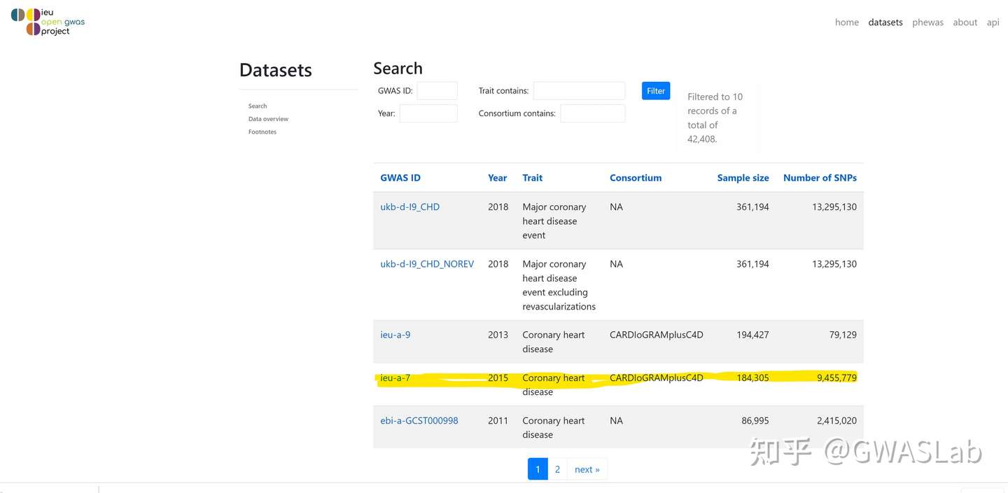
例如我们想分析BMI与冠心病（coronary heart disease）之间的因果关系，首先我们要查找冠心病GWAS在数据库中的id

2.1 查找相应的GWAS

使用available_outcomes()可以查看当前可用的所有表型的GWAS数据，然后使用grep1抓取关键字

ao <- available_outcomes()
#> API: public: <http://gwas-api.mrcieu.ac.uk/>
head(ao)
#> # A tibble: 6 x 22
#>   id      trait     group_name  year consortium author sex   population    unit 
#>   <chr>   <chr>     <chr>      <int> <chr>      <chr>  <chr> <chr>         <chr>
#> 1 ieu-b-~ Number o~ public      2021 MRC-IEU    Clare~ Male~ European      SD   
#> 2 prot-a~ Leptin r~ public      2018 NA         Sun BB Male~ European      NA   
#> 3 prot-a~ Adapter ~ public      2018 NA         Sun BB Male~ European      NA   
#> 4 ukb-e-~ Impedanc~ public      2020 NA         Pan-U~ Male~ Greater Midd~ NA   
#> 5 prot-a~ Dual spe~ public      2018 NA         Sun BB Male~ European      NA   
#> 6 eqtl-a~ ENSG0000~ public      2018 NA         Vosa U Male~ European      NA   
#> # ... with 13 more variables: sample_size <int>, nsnp <int>, build <chr>,
#> #   category <chr>, subcategory <chr>, ontology <chr>, note <chr>, mr <int>,
#> #   pmid <int>, priority <int>, ncase <int>, ncontrol <int>, sd <dbl>

## 使用grep1抓取目标表型
ao[grepl("heart disease", ao$trait), ]
#> # A tibble: 28 x 22
#>    id      trait       group_name  year consortium author sex   population unit 
#>    <chr>   <chr>       <chr>      <int> <chr>      <chr>  <chr> <chr>      <chr>
#>  1 ieu-a-8 Coronary h~ public      2011 CARDIoGRAM Schun~ Male~ European   log ~
#>  2 finn-a~ Valvular h~ public      2020 NA         NA     Male~ European   NA   
#>  3 finn-a~ Other or i~ public      2020 NA         NA     Male~ European   NA   
#>  4 ukb-b-~ Diagnoses ~ public      2018 MRC-IEU    Ben E~ Male~ European   SD   
#>  5 ukb-a-~ Diagnoses ~ public      2017 Neale Lab  Neale  Male~ European   SD   
#>  6 ukb-e-~ I25 Chroni~ public      2020 NA         Pan-U~ Male~ South Asi~ NA   
#>  7 ukb-b-~ Diagnoses ~ public      2018 MRC-IEU    Ben E~ Male~ European   SD   
#>  8 finn-a~ Ischemic h~ public      2020 NA         NA     Male~ European   NA   
#>  9 finn-a~ Major coro~ public      2020 NA         NA     Male~ European   NA   
#> 10 finn-a~ Other hear~ public      2020 NA         NA     Male~ European   NA   
#> # ... with 18 more rows, and 13 more variables: sample_size <int>, nsnp <int>,
#> #   build <chr>, category <chr>, subcategory <chr>, ontology <chr>, note <chr>,
#> #   mr <int>, pmid <int>, priority <int>, ncase <int>, ncontrol <int>, sd <dbl>

查看完整结果后我们发现冠心病GWAS id为 ieu-a-7

当然可以直接进入数据库网站搜索 https://gwas.mrcieu.ac.uk/ ，简单直观

2.2 提取结局GWAS数据

指定GWAS id，指定要提取的SNP rsid （1中选取的工具变量），使用extract_outcome_data进行提取

chd_out_dat <- extract_outcome_data(
    snps = bmi_exp_dat$SNP,
    outcomes = 'ieu-a-7'
)

head(chd_out_dat )
A data.frame: 6 × 16
SNP	chr	pos	beta.outcome	se.outcome	samplesize.outcome	pval.outcome	eaf.outcome	effect_allele.outcome	other_allele.outcome	outcome	id.outcome	originalname.outcome	outcome.deprecated	mr_keep.outcome	data_source.outcome
<chr>	<chr>	<chr>	<dbl>	<dbl>	<dbl>	<dbl>	<dbl>	<chr>	<chr>	<chr>	<chr>	<chr>	<chr>	<lgl>	<chr>
1	rs887912	2	59302877	-0.021960	0.0111398	184305	0.04868780	0.731654	C	T	Coronary heart disease || id:ieu-a-7	ieu-a-7	Coronary heart disease	Coronary heart disease || ||	TRUE	igd
2	rs2112347	5	75015242	-0.005855	0.0096581	184305	0.54436400	0.401399	G	T	Coronary heart disease || id:ieu-a-7	ieu-a-7	Coronary heart disease	Coronary heart disease || ||	TRUE	igd
3	rs3817334	11	47650993	0.000355	0.0095386	184305	0.97031200	0.387831	T	C	Coronary heart disease || id:ieu-a-7	ieu-a-7	Coronary heart disease	Coronary heart disease || ||	TRUE	igd
4	rs1555543	1	96944797	0.002516	0.0093724	184305	0.78835500	0.558318	C	A	Coronary heart disease || id:ieu-a-7	ieu-a-7	Coronary heart disease	Coronary heart disease || ||	TRUE	igd
5	rs2815752	1	72812440	0.010402	0.0098384	184305	0.29038200	0.611282	A	G	Coronary heart disease || id:ieu-a-7	ieu-a-7	Coronary heart disease	Coronary heart disease || ||	TRUE	igd
6	rs10938397	4	45182527	0.030606	0.0093485	184305	0.00106079	0.416076	G	A	Coronary heart disease || id:ieu-a-7	ieu-a-7	Coronary heart disease	Coronary heart disease || ||	TRUE	igd

3 对数据进行预处理，使其效应等位与效应量保持统一

完成暴露因素与结局GWAS数据的提取后，我们要对其进行预处理，使其效应等位保持统一，可以使用harmonise_data函数，方便的完成处理：

dat <- harmonise_data(
    exposure_dat = bmi_exp_dat, 
    outcome_dat = chd_out_dat
)

到这一步数据的准备工作就完成了，下一步可以开始分析

4 MR分析与可视化

4.1 MR分析

使用mr函数对处理好的数据dat 进行分析，结果如下

res <- mr(dat)
#> Analysing 'ieu-a-2' on 'ieu-a-7'
res
#>   id.exposure id.outcome                              outcome
#> 1     ieu-a-2    ieu-a-7 Coronary heart disease || id:ieu-a-7
#> 2     ieu-a-2    ieu-a-7 Coronary heart disease || id:ieu-a-7
#> 3     ieu-a-2    ieu-a-7 Coronary heart disease || id:ieu-a-7
#> 4     ieu-a-2    ieu-a-7 Coronary heart disease || id:ieu-a-7
#> 5     ieu-a-2    ieu-a-7 Coronary heart disease || id:ieu-a-7
#>                        exposure                    method nsnp         b
#> 1 Body mass index || id:ieu-a-2                  MR Egger   79 0.5024935
#> 2 Body mass index || id:ieu-a-2           Weighted median   79 0.3870065
#> 3 Body mass index || id:ieu-a-2 Inverse variance weighted   79 0.4459091
#> 4 Body mass index || id:ieu-a-2               Simple mode   79 0.3401554
#> 5 Body mass index || id:ieu-a-2             Weighted mode   79 0.3888249
#>           se         pval
#> 1 0.14396056 8.012590e-04
#> 2 0.07226598 8.541141e-08
#> 3 0.05898302 4.032020e-14
#> 4 0.15698810 3.330579e-02
#> 5 0.09240475 6.833558e-05

mr默认使用五种方法（ MR Egger，Weighted median，Inverse variance weighted，Simple mode ，Weighted mode ）

但我们可以额外指定方法,使用mr_method_list()查看当前支持的统计方法

mr_method_list()

obj	name	PubmedID	Description	use_by_default	heterogeneity_test
<chr>	<chr>	<chr>	<chr>	<lgl>	<lgl>
mr_wald_ratio	Wald ratio			TRUE	FALSE
mr_two_sample_ml	Maximum likelihood			FALSE	TRUE
mr_egger_regression	MR Egger	26050253		TRUE	TRUE
mr_egger_regression_bootstrap	MR Egger (bootstrap)	26050253		FALSE	FALSE
mr_simple_median	Simple median			FALSE	FALSE
mr_weighted_median	Weighted median			TRUE	FALSE
mr_penalised_weighted_median	Penalised weighted median			FALSE	FALSE
mr_ivw	Inverse variance weighted			TRUE	TRUE
mr_ivw_radial	IVW radial			FALSE	TRUE
mr_ivw_mre	Inverse variance weighted (multiplicative random effects)			FALSE	FALSE
mr_ivw_fe	Inverse variance weighted (fixed effects)			FALSE	FALSE
mr_simple_mode	Simple mode			TRUE	FALSE
mr_weighted_mode	Weighted mode			TRUE	FALSE
mr_weighted_mode_nome	Weighted mode (NOME)			FALSE	FALSE
mr_simple_mode_nome	Simple mode (NOME)			FALSE	FALSE
mr_raps	Robust adjusted profile score (RAPS)			FALSE	FALSE
mr_sign	Sign concordance test		Tests for concordance of signs between exposure and outcome	FALSE	FALSE
mr_uwr	Unweighted regression		Doesn't use any weights	FALSE	TRUE

在mr函数中，添加想要使用的方法即可：

mr(dat, method_list=c("mr_egger_regression", "mr_ivw"))
#> Analysing 'ieu-a-2' on 'ieu-a-7'
#>   id.exposure id.outcome                              outcome
#> 1     ieu-a-2    ieu-a-7 Coronary heart disease || id:ieu-a-7
#> 2     ieu-a-2    ieu-a-7 Coronary heart disease || id:ieu-a-7
#>                        exposure                    method nsnp         b
#> 1 Body mass index || id:ieu-a-2                  MR Egger   79 0.5024935
#> 2 Body mass index || id:ieu-a-2 Inverse variance weighted   79 0.4459091
#>           se        pval
#> 1 0.14396056 8.01259e-04
#> 2 0.05898302 4.03202e-14

4.2 敏感性分析

4.2.1 异质性检验 mr_heterogeneity

mr_heterogeneity(dat)
#>   id.exposure id.outcome                              outcome
#> 1     ieu-a-2    ieu-a-7 Coronary heart disease || id:ieu-a-7
#> 2     ieu-a-2    ieu-a-7 Coronary heart disease || id:ieu-a-7
#>                        exposure                    method        Q Q_df
#> 1 Body mass index || id:ieu-a-2                  MR Egger 143.3046   77
#> 2 Body mass index || id:ieu-a-2 Inverse variance weighted 143.6508   78
#>         Q_pval
#> 1 6.841585e-06
#> 2 8.728420e-06

4.2.2 水平多效性检验 mr_pleiotropy_test

MR Egger 回归中的截距是反应水平多效性的一个有效指标，可以通过mr_pleiotropy_test计算

mr_pleiotropy_test(dat)
#>   id.exposure id.outcome                              outcome
#> 1     ieu-a-2    ieu-a-7 Coronary heart disease || id:ieu-a-7
#>                        exposure egger_intercept          se      pval
#> 1 Body mass index || id:ieu-a-2    -0.001719304 0.003985962 0.6674266

4.3 可视化

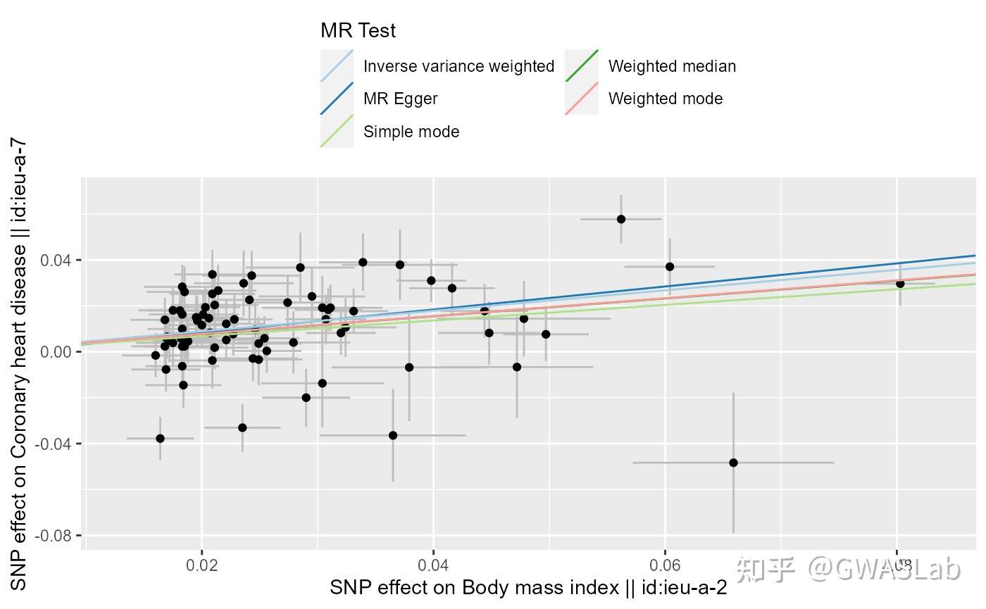
4.3.1 散点图

对上述的MR结果与输入数据，使用mr_scatter_plot函数绘制散点图

res <-mr(dat)
#> Analysing 'ieu-a-2' on 'ieu-a-7'
p1 <-mr_scatter_plot(res, dat)

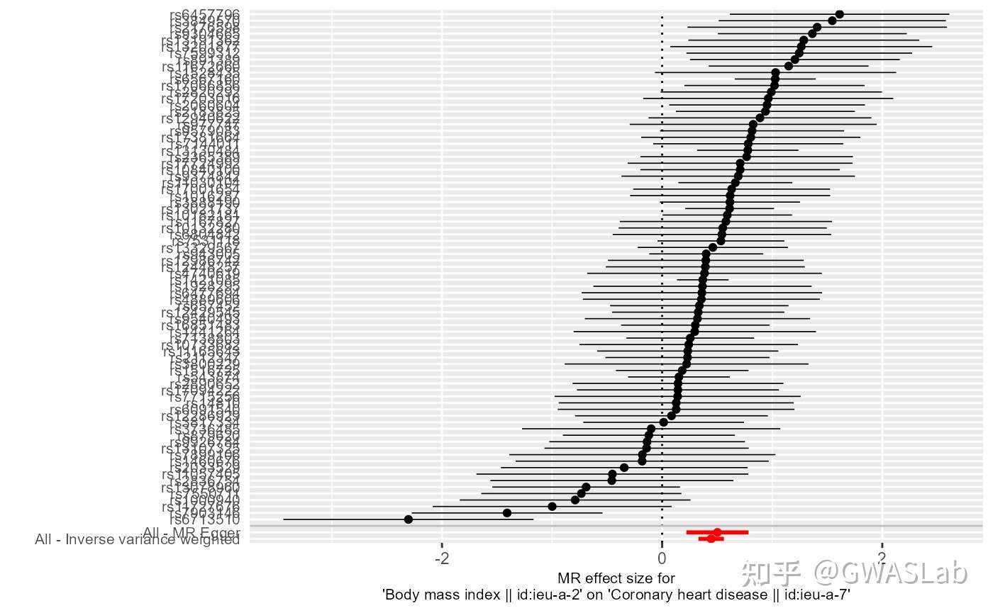
4.3.2 森林图

首先使用mr_singlesnp获取单个SNP的结果，然后使用mr_forest_plot绘制森林图

res_single <- mr_singlesnp(dat)
p2 <- mr_forest_plot(res_single)
p2[[1]]
#> Warning: Removed 1 rows containing missing values (geom_errorbarh).
#> Warning: Removed 1 rows containing missing values (geom_point).

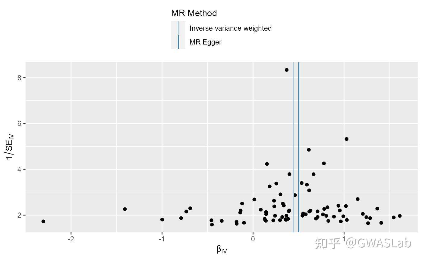
4.3.2 漏斗图

首先使用mr_singlesnp获取单个SNP的结果，然后使用mr_funnel_plot绘制漏斗图

res_single <- mr_singlesnp(dat)
p4 <- mr_funnel_plot(res_single)
p4[[1]]

参考：

Hemani G, Tilling K, Davey Smith G (2017) Orienting the causal relationship between imprecisely measured traits using GWAS summary data. PLOS Genetics 13(11): e1007081. https://doi.org/10.1371/journal.pgen.1007081

Hemani G, Zheng J, Elsworth B, Wade KH, Baird D, Haberland V, Laurin C, Burgess S, Bowden J, Langdon R, Tan VY, Yarmolinsky J, Shihab HA, Timpson NJ, Evans DM, Relton C, Martin RM, Davey Smith G, Gaunt TR, Haycock PC, The MR-Base Collaboration. The MR-Base platform supports systematic causal inference across the human phenome. eLife 2018;7:e34408. doi: 10.7554/eLife.34408

https://mrcieu.github.io/TwoSam

本文是MR系列的第一篇，孟德尔随机化的简介，该系列会介绍孟德尔随机化的基础概念，统计方法分类，常见误区与实践操作等内容。

1.背景与目的
- 1.1 明确因果关系
- 1.2 RCT是金标准，但缺点明显
- 1.3 孟德尔随机化的本质
2.孟德尔随机化的统计学方法 – 工具变量
3.核心假设
- 3.1 关联性假设
- 3.2 排他性限制
- 3.3 独立性假设
4.孟德尔随机化的优势

1 背景与目的

1.1目的是明确因果关系

在关联分析中我们时常面对的一个问题便是我们很难确定一个变量是否是真正的因果变量，而非有其他未观测的因素同时影响这个变量与结果，造成这个变量与结果相关联。在循证医学中，或是制定干预策略时，明确因果性是十分必要的。

这个问题实际上与内生性 endogeneity 相关，包括：反向因果关系 reverse causation, 忽略的混淆变量造成的偏倚 omitted variable bias due to confounding, 测量误差measurement error, 以及双向因果关系bidirectional causality等等问题。（这里的内生性在统计学上是指在回归分析中，解释变量（x）与误差项相关。）

1.2. RCT是金标准，但缺点明显

一般来说，明确因果关系的金标准时随机对照试验 RCT randomized control trial (RCT)，即对受试者随机分为对照组和实验组，以研究某个因素的影响。但现实中，要完成随机对照试验的难度非常高，需要大量的人力物力，有时因为伦理问题，对某个因素的研究几乎是不可能的。这时我们就要借助其他方法，而孟德尔随机化就是其中之一。

1.3. 孟德尔随机化与RCT的相似性

孟德尔随机化（MR，Mendelian randomization）便是为了解决以上问题而开发的方法，MR与RCT直接相关，两者有很高的相似性，如下图所示。

孟德尔随机化的核心其实是利用了孟德尔第二定律，也就是自由组合规律(law of independent assortment），当具有两对（或更多对）相对性状的亲本进行杂交，在子一代产生配子时，在等位基因分离的同时，非同源染色体上的基因表现为自由组合，这一过程类似于随机对照试验中的随机分组，所以我个人理解的孟德尔随机化就是基于孟德尔第二定律的随机对照试验。

2 孟德尔随机化的统计学方法 – 工具变量

孟德尔随机化在统计学上的本质实际是利用工具变量（Instrumental variables）来研究因果性，这一方法常用在经济学研究中。

工具变量简单来说就是，一个与X相关，但与被忽略的混淆因素以及Y不相关的变量。在经济学研究中工具变量可以是政策改革，自然灾害等等，而在遗传学中，这个变量就是基因。

如果一个基因变异Z 是某个暴露因素X的因果变量，并且对结果Y没有直接因果关系，那么这个基因变异Z与结果Y的关联，只能通过X对Y的因果关系而被观察到（X->Y）。

2.1 两阶段最小二乘法

通常我们可以用两阶段最小二乘法（2SLS，2 stage least squared method）来估计X对Y的效应：

考虑一种最简单的单样本的情况，有一个基因变异Z，与Z相关的因素X，以及与Z不相关的结果Y，

我们想探究X与Y之间的因果关系。

第一阶段，X对工具变量进行回归，

第二阶段，Y对第一阶段X的预测值进行回归，

合并后可以化为Y直接对工具变量进行回归。

我们所关心的系数β2SLS实际上也等同于两段协方差的比值

2.2 两样本MR

另一种常见的情况则是两样本MR，如果我们有一个与X相关联的工具变量，我们只有在X对Y有因果关系的情况下，才能观测到这个工具变量与Y的关联。

这意味着βiv,y = βiv,x 乘以 βx,y。也就是说，我们可以不用通过X与Y的回归来估计β，

而是可以简单地通过 βx,y = βiv,y / βiv,x 来计算 X对Y的效应量。

这就意味着与两阶段最小二乘法相对，我们可以利用两个独立的GWAS 的概括性统计量来计算这个比值。这种方法通常叫做两样本MR.

当然MR还有其他更复杂的统计模型方法，这里不做深究，有兴趣的朋友的可以看这篇文章：预留链接

核心假设：

当然，既然是统计模型那就要满足模型的基本假设，通常情况下MR建立在几点基本假设之上，

主要假设：

3.1 遗传变异必须与暴露因素X强相关。（关联性假设），例如：弱工具变量的使用会导致估计出现偏倚。

3.2 遗传变异不能与结果直接相关。(排他性限制)，例如：可能影响因素包括多效性等。

3.3 遗传变异不能与任何可能的混淆因素相关 (独立性假设)，例如：人群分层

其他假设：

3.4 不存在选型交配 No genetic assortative mating，例如：人们经常会与自己教育和经济水平相似的人结婚。

3.5 对所有个体，IV对于X的影响方向是相同的。例如：潜在的上位效应与GxE基因与环境的相互作用都可能会影响此假设。

总结来看，孟德尔随机化以基因型作为工具变量的优势是：

4.1 遗传相关中，因果关系的方向是确定的，遗传多样性导致了不同的表型，反之则不成立

4.2 一般情况下我们所测量的环境暴露因素都或多或少与行为，社会，心理等因素相关，造成偏倚。但遗传变异则不受这些混淆因素影响。

4.3 相对来说，遗传变异与其效应的测量误差较小。

4.4 并不一定要找到因果SNP，一个与因果SNP处于LD的SNP即可满足假设条件。

4.5.目前GWAS的数据相对容易获取。

参考：

Melinda C. Mills, Nicola Barban, and F. C. T. An Introduction to Statistical Genetic Data Analysis. (2020).

Curr Epidemiol Rep . 2017;4(4):330-345. doi: 10.1007/s40471-017-0128-6. Epub 2017 Nov 22.

分类： 09 孟德尔随机化 Mendelian randomization

孟德尔随机化系列之二：两样本MR – TwoSampleMR