GWAS 全基因组关联分析 – 第 4 页 – GWASLab

major/minor/reference/alternative/risk/effect allele 概念解析

这些名词很容易混淆而引起不必要的错误或误解，早期的遗传统计学软件，例如plink并没有很重视allele概念上的明确区分，但近年新出的软件或旧软件的新版本为保证统一性已经开始注意此问题。

本文内容

第一组 频率上的 major 与 minor allele 
第二组 参考基因组的 reference （ref） 与 alternative （alt） allele
第三组 关联检验的 reference （non-risk 或者 non-effect）与 risk/effect allele

首先第一组概念 major 与 minor allele

major allele 与 minor allele 通常针对某一大小确定的特定群体而言，频率最高的allele为该群体的major allele，频率次高的为 minor allele，对于最常见的bi-allelic SNP来说，两个allele频率一高一低，就是这个群体中这个snp的major和minor allele，对于tri- 或者quad-allelic SNP （位点有三种或四种碱基的SNP）而言，minor allele则是频率第二高的那个allele

注意点：

区分major与minor的依据是 某一大小确定特定群体的 allele 频率

plink1.9目前采用的是major与minor allele的概念，软件会自动计算频率，对原始数据进行操作时会自动改变allele的排序，如果你使用plink1.9 的—frq选项计算频率，你会发现输出的文件中是MAF ，minor allele frequency，不会高于0.5。

PLINK1.9中,A1为minor，A2为major allele，所以这里MAF是指A1（minor allele）的频率。。

CHR    SNP    A1   A2          MAF  NCHROBS
1      SNP1    T    C       0.1258    10000
1      SNP2    A    G       0.1258    10000

第二组 reference （ref）与 alternative （alt） allele

reference allele 在这里是指某一参考基因组上该位点的allele，该位点上其他的allele则称为alternative allele。注意，这里reference 与 alternative allele与频率无关，唯一的决定因素是所选的参考基因组。参考基因组上的allele多为major allele，但这只是巧合，不能以此为依据将major和 reference allele划上等号，也有部分reference allele在该群体中为minor allele。

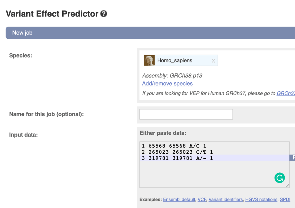
与plink1.9不同，plink2使用的概念则是reference 与 alternative allele，进行操作时不会自动依据频率而改变ref与alt的排序，使用plink2 的—frq选项计算频率，你会发现输出的文件中是alternative allele frequency (不是MAF)，取值范围为[0,1]。

PLINK2中则明确区分了reference 与 alternative allele的概念，例如上述的两个SNP，根据参考基因组对齐后，SNP1在参考基因组中的ref为T，那么alt就为C，这里计算的alt的频率为0.8742，按概念来说在该群体中，SNP1的T为ref allele，但却又是minor allele ，而C为alt，却又是major。对于SNP2来说ref 则为 major，alt 为minor。

#CHROM	ID	REF	ALT	ALT_FREQS	OBS_CT
1	SNP1    	T	C	0.8742	10000
1	SNP2    	G	A	0.1258	10000

小窍门：使用plink2可以将自己手头数据的ref与alt allele与对应参考基因组对齐，示例代码如下：

plink2 \
       --bfile testfile \
       --ref-from-fa -fa hg19.fasta \  从参考基因组的fasta文件来决定plink文件中的ref
       --make-bed \
       --out testfile_fa

第三组 reference 与 risk/effect allele

在这里的概念再次改变，同样的reference allele，在与 risk/effect allele并列时，则指的是GWAS关联检测中的reference allele （non-risk 或者 non-effect），也就是效应量beta（或odds ratio）估计时的对比的参考（reference group），但有的软件也会将 reference allele 作为 effect allele。其概念上与上述ref与alt的组合无关，但为了保持统一性，近年来研究中关联检验的reference 也会与 reference genome保持一致，以避免混淆等。（注意：早期多以minor allele为关联检验的ref allele，这也是容易产生混淆的点）。reference allele的概念非常混乱，辨别时不要拘泥于名称，要关注具体效应量的指代。

risk allele 则很好理解，就是对疾病发生有贡献的那个allele，在复杂疾病的研究中，一般情况下risk allele经常为minor allele，但也会有例外。effect allele的概念也类似，就是我们想要研究其对疾病或表型效应的allele，所以通常是对表型或疾病有贡献的allele，关联检验结果中effect一栏指的就是effect allele的效应。

理解了以上概念后，我们在分辨allele时就能得心应手了。

多基因风险分数 PRS( Polygenic risk score)系列之二：使用PLINK计算PRS（C+T方法）

本文内容

简介
第1步 事先准备
第2步 clumping
第3步 使用PLINK计算PRS
第4步 寻找最佳的P值阈值
参考

简介：

PRS基础回顾 :多基因风险分数 PRS( Polygenic risk score)系列之一：概念入门

PLINK是群体遗传学研究中一款非常强大的软件，尽管PLINK并不是专门为计算PRS而开发，但其内置的功能足以使我们完成C+T （clumping + p value thresholding，也称P + T）计算PRS方法必要的步骤，在初学阶段对于理解PRS计算过程有很大帮助。本文将简要介绍使用PLINK计算PRS的过程（本教程改编自https://choishingwan.github.io/PRS-Tutorial/plink/ ）：

本文所用数据（已经完成QC）：

下载链接，由教程原作者提供：

https://drive.google.com/file/d/1x_G0Gxk9jFMY-PMqwtg6-vdEyUPp5p5u/view

也可以使用自己准备的数据，必要的数据包括

1 target样本的plink文件 (bed,bim,fam)
2 base样本的GWAS概括性数据 
3 target样本的表型数据

第1步事前准备：更新效应量

当表型为二变量表型时，SNP的效应量通常表示为odds ratio（OR），这种情况下计算PRS时要计算乘积，这里为了简化我们将OR转化为beta，就可以只计算加和。

head Height.QC
CHR	BP	SNP	A1	A2	N	SE	P	OR	INFO	MAF
1	756604	rs3131962	A	G	388028	0.00301666	0.483171	0.997886915712650.890557941364774	0.369389592764921
1	768448	rs12562034	A	G	388028	0.00329472	0.834808	1.000687316093530.895893511351165	0.336845754096289
1	779322	rs4040617	G	A	388028	0.00303344	0.42897	0.997603556067569	0.897508290615237	0.377368010940814
1	801536	rs79373928	G	T	388028	0.00841324	0.808999	1.002035699227930.908962856432993	0.483212245374095
1	808631	rs11240779	G	A	388028	0.00242821	0.590265	1.001308325111540.893212523690488	0.450409558999587
1	809876	rs57181708	G	A	388028	0.00336785	0.71475	1.00123165786833	0.923557624081969	0.499743932656759
1	835499	rs4422948	G	A	388028	0.0023758	0.710884	0.999119752645200.906437735120596	0.481016005816168
1	838555	rs4970383	A	C	388028	0.00235773	0.150993	0.996619945289750.907716506801574	0.327164029672754
1	840753	rs4970382	C	T	388028	0.00207377	0.199967	0.997345678956140.914602590137255	0.498936220426316

可以利用简单的R脚本进行转换，在这里我们在文件的最后一列后添加转换后的beta

dat <- read.table(gzfile("Height.QC.gz"), header=T)
dat$BETA <- log(dat$OR)
write.table(dat, "Height.QC.Transformed", quote=F, row.names=F)
q() # exit R

将OR转换成beta后

head Height.QC.Transformed
CHR BP SNP A1 A2 N SE P OR INFO MAF BETA
1 756604 rs3131962 A G 388028 0.00301666 0.483171 0.997886915712657 0.890557941364774 0.369389592764921 -0.00211532000000048
1 768448 rs12562034 A G 388028 0.00329472 0.834808 1.00068731609353 0.895893511351165 0.336845754096289 0.000687079999998082
1 779322 rs4040617 G A 388028 0.00303344 0.42897 0.997603556067569 0.897508290615237 0.377368010940814 -0.00239932000000021
1 801536 rs79373928 G T 388028 0.00841324 0.808999 1.00203569922793 0.908962856432993 0.483212245374095 0.00203362999999797
1 808631 rs11240779 G A 388028 0.00242821 0.590265 1.00130832511154 0.893212523690488 0.450409558999587 0.00130747000000259
1 809876 rs57181708 G A 388028 0.00336785 0.71475 1.00123165786833 0.923557624081969 0.499743932656759 0.00123090000000354
1 835499 rs4422948 G A 388028 0.0023758 0.710884 0.999119752645202 0.906437735120596 0.481016005816168 -0.000880634999999921
1 838555 rs4970383 A C 388028 0.00235773 0.150993 0.996619945289758 0.907716506801574 0.327164029672754 -0.0033857799999997
1 840753 rs4970382 C T 388028 0.00207377 0.199967 0.99734567895614 0.914602590137255 0.498936220426316 -0.00265785000000019

第2步 Clumping （基于P值的LD-pruning）

回顾：SNP的LD剪枝与聚集 LD pruning & clumping

plink \
    --bfile EUR.QC \
    --clump-p1 1 \
    --clump-r2 0.1 \
    --clump-kb 250 \
    --clump Height.QC.Transformed \
    --clump-snp-field SNP \
    --clump-field P \
    --out EUR

其中

–bfile 是输入的PLINK格式文件（target样本）

–clump 则为GWAS的包含P值的概括性数据（base样本）

--clump-p1 1 \
	该选项依据P值，对索引SNP（每个clump中心的SNP）施加过滤，默认值为0.0001
--clump-r2 0.1 \
	与索引SNP的r2大于0.1的位点被归于与索引SNP为同一clump，在计算时去除
--clump-kb 250 \
	进行clumping时只考虑与索引SNP的距离小于250 kb的位点
--clump-snp-field SNP \
	概括性数据文件中变异ID的列名
--clump-field P \
	概括性数据文件中表示P值的列名

详细文档可参考：https://www.cog-genomics.org/plink/1.9/postproc#clump

执行以上命令后我们会得到文件 EUR.clumped，该文件包含clumping后的索引SNP。

head EUR.clumped
CHR    F         SNP         BP        P    TOTAL   NSIG    S05    S01   S001  S0001    SP2
   6    1   rs3134762   31210866  4.52e-165      180     20      0      0      0    160 rs2523898(1),rs13210132(1),rs28732080(1),rs28732081(1),rs28732082(1),rs2517552(1),rs2517546(1),rs2844647(1),rs2517537(1),rs2844645(1),rs2523857(1),rs2517527(1),rs3131788(1),rs3132564(1),rs3130955(1),rs3130544(1),rs2535296(1),rs2517448(1),rs6457327(1),rs28732096(1),rs2233956(1),rs1265048(1),rs3130985(1),rs13201757(1),rs6909321(1),rs3130557(1),rs17196961(1),rs9501055(1),rs13200022(1),rs3130573(1),rs28732101(1),rs1265095(1),rs2233940(1),rs130079(1),rs746647(1),rs2240064(1),rs3131012(1)...

我们可以通过以下代码提取这些SNP的id, 用于下一步计算

awk 'NR!=1{print $3}' EUR.clumped > EUR.valid.snp

注意：

这里的r2计算是基于最大似然单倍型频率估计的，如果你的target样本比较少（<500），那么计算LD的r2时最好使用千人基因组项目中相应群体的数据。

第3步计算 PRS

plink提供了—score选项，是我们可以方便的计算PRS

需要以下输入文件：

base样本的GWAS概括性数据文件 Height.QC.Transformed
一个包含SNP ID与相应P值的文件
使用awk命令从Height.QC.Transformed中提取SNPID与P值即可
awk ‘{print $3,$8}’ Height.QC.Transformed > SNP.pvalue

在这里我们计算多个P值范围内SNP的PRS

echo "0.001 0 0.001" > range_list 
echo "0.05 0 0.05" >> range_list
echo "0.1 0 0.1" >> range_list
echo "0.2 0 0.2" >> range_list
echo "0.3 0 0.3" >> range_list
echo "0.4 0 0.4" >> range_list
echo "0.5 0 0.5" >> range_list

上述范围的三个数字分别为，名称，范围的下限，范围的上限

例如0.001 0 0.001 ，名称为0.001的这个范围，下限为0，上限为0.0001

下面开始计算，PLINK代码如下

plink \
    --bfile EUR.QC \
    --score Height.QC.Transformed 3 4 12 header \
    --q-score-range range_list SNP.pvalue \
    --extract EUR.valid.snp \
    --out EUR

其中 –q-score-range 即为包含P值范围的文件与一个包含SNP ID与相应P值的文件

–score 为计算分数的选项，3, 4，12 分别表示SNP ID，allele code与beta 分别在文件的第 3， 4， 12列， header表示输入文件有表头。

当然在计算时也可以加入协变量，例如PC等，这里就略过

执行后输出对应上述7个范围的PRS的文件：

EUR.0.5.profile
EUR.0.4.profile
EUR.0.3.profile
EUR.0.2.profile
EUR.0.1.profile
EUR.0.05.profile
EUR.0.001.profile

head EUR.0.001.profile
FID       IID  PHENO    CNT   CNT2    SCORE
  HG00096   HG00096     -9  32678   6894 -4.41148e-05
  HG00097   HG00097     -9  32678   6921 5.71558e-05
  HG00099   HG00099     -9  32678   6759 7.23017e-07
  HG00101   HG00101     -9  32678   6875 3.48096e-05
  HG00102   HG00102     -9  32678   6966 4.68491e-05
  HG00103   HG00103     -9  32678   6763 8.78172e-05
  HG00105   HG00105     -9  32678   6960 4.39891e-05
  HG00107   HG00107     -9  32678   6835 2.45655e-05
  HG00108   HG00108     -9  32678   6884 7.68976e-05

第4步寻找 best-fit PRS

通常情况下，事先我们并不知道最优的P值阈值，所以在计算完成多组PRS后，为了找到最适阈值，需要对PRS进行回归分析，然后选取能够解释最多表型方差的P值阈值。

示例R代码如下 bestfit.R

p.threshold <- c(0.001,0.05,0.1,0.2,0.3,0.4,0.5)
# Read in the phenotype file 
phenotype <- read.table("EUR.height", header=T)
# Read in the PCs
pcs <- read.table("EUR.eigenvec", header=F)
# The default output from plink does not include a header
# To make things simple, we will add the appropriate headers
# (1:6 because there are 6 PCs)
colnames(pcs) <- c("FID", "IID", paste0("PC",1:6)) 
# Read in the covariates (here, it is sex)
covariate <- read.table("EUR.cov", header=T)
# Now merge the files
pheno <- merge(merge(phenotype, covariate, by=c("FID", "IID")), pcs, by=c("FID","IID"))
# We can then calculate the null model (model with PRS) using a linear regression 
# (as height is quantitative)
null.model <- lm(Height~., data=pheno[,!colnames(pheno)%in%c("FID","IID")])
# And the R2 of the null model is 
null.r2 <- summary(null.model)$r.squared
prs.result <- NULL
for(i in p.threshold){
    # Go through each p-value threshold
    prs <- read.table(paste0("EUR.",i,".profile"), header=T)
    # Merge the prs with the phenotype matrix
    # We only want the FID, IID and PRS from the PRS file, therefore we only select the 
    # relevant columns
    pheno.prs <- merge(pheno, prs[,c("FID","IID", "SCORE")], by=c("FID", "IID"))
    # Now perform a linear regression on Height with PRS and the covariates
    # ignoring the FID and IID from our model
    model <- lm(Height~., data=pheno.prs[,!colnames(pheno.prs)%in%c("FID","IID")])
    # model R2 is obtained as 
    model.r2 <- summary(model)$r.squared
    # R2 of PRS is simply calculated as the model R2 minus the null R2
    prs.r2 <- model.r2-null.r2
    # We can also obtain the coeffcient and p-value of association of PRS as follow
    prs.coef <- summary(model)$coeff["SCORE",]
    prs.beta <- as.numeric(prs.coef[1])
    prs.se <- as.numeric(prs.coef[2])
    prs.p <- as.numeric(prs.coef[4])
    # We can then store the results
    prs.result <- rbind(prs.result, data.frame(Threshold=i, R2=prs.r2, P=prs.p, BETA=prs.beta,SE=prs.se))
}
# Best result is:
prs.result[which.max(prs.result$R2),]
q() # exit R

执行后就可以看到本次PRS计算中，最优的阈值为0.3

Rscript bestfit.R 
  Threshold        R2            P     BETA       SE
5       0.3 0.1638468 1.025827e-25 47343.32 4248.152

参考：

Basic Tutorial for Polygenic Risk Score Analyses

HLA系统命名规则

本文内容：

背景
HLA简介
命名规则 Nomenclature
一些特殊标记
HLA分型的解析度 Resolution
参考

背景

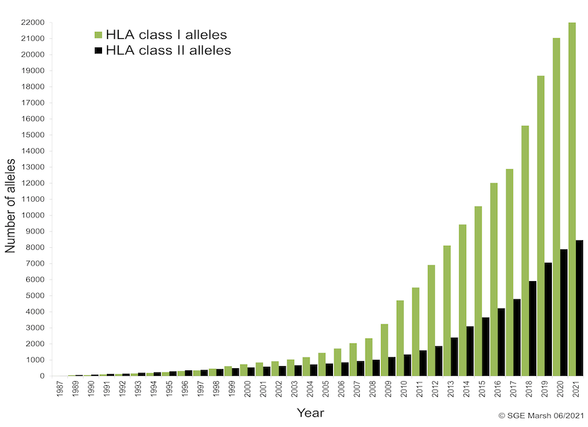
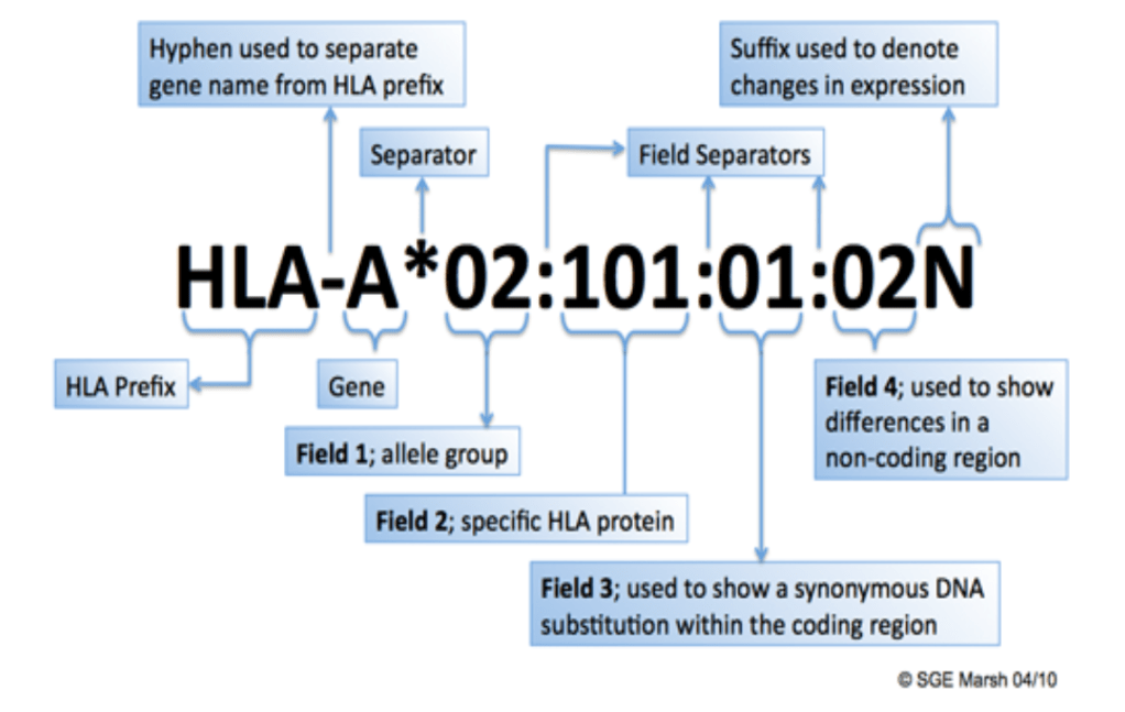
WHO的 Nomenclature Committee for Factors of the HLA System 为了区分编码HLA分子的HLA等位基因，于1987年开始施行4位数字的命名方法。后在2002年，由于4位数字的命名法已经不再适应该领域的快速发展，遂将HLA-A*02 群改为 A*92，将HLA-B15改为B95进行管理。但近年随着等位基因数的不断增加，其他的抗原群也难以在现行命名规则下管理。于是在2010年，发布了现行的HLA等位基因命名规则。这次变更后，使用冒号“：”分隔表示不同HLA等位基因的4个数字区域，并取消了固定位数的限制。

已发现的HLA等位基因数量逐年增加：

HLA基础：推荐 https://zhuanlan.zhihu.com/p/382011751 ，简单易懂

命名规则如下图所示：

HLA为前缀，A表示基因，使用星号*与4个数字区域进行分割。

被冒号“：”分隔的四个数字区域分别标示以下内容：

・第 1 区域：相关联的血清学HLA分型，或是该等位基因所属的等位基因组（例：A*02，A*03，A*11，C*03 等）
・第 2 区域：同一血清学 HLA 型或是等位基因组内，伴随氨基酸变异的等位基因（亚型）（例：A*02:02，A*02:04，A*02:07等）

・第 3 区域：不伴随氨基酸变异的等位基因（同义置换：synonymous DNA substitution）（例：A*02:01:02，A*02:01:03，A*02:01:04 等）
・第 4 区域：非编码区域伴随碱基置换的等位基因（例：A*02:01:01:01，A*02:01:01:02L，A*02:01:01:03 等）

一些特殊标记：

存在两种以上等位基因无法判定时使用 / 分隔，例如：HLA-DRB1*15/16
无法判定的等位基因过多时，使用+表示省略，例如：HLA-DRB1*15:01/16:01/+
表示肽链结合区（HLA class I：exon2 和3，HLA class II ：exon2）的不确定性时，氨基酸序列（P），或是碱基序列（G）一致的等位基因，在末尾添加P或G表示。例如：A02:01:01:01/02:01:01:02L/02:01:01:03/02:01:02/02:01:03/02:01:04/02:01:05/02:01:06/02:01:07/02:01:08/02:01:09/02:01:10/02:01:11/02:01:12/02:01:13/02:01:14/02:01:15/02:01:17/02:01:18/02:01:19/02:01:21/02:01:22/02:09/02:66/02:75/02:89/02:97/02:132/02:134/02:140 可以表示为 A02:01P
N: Null alleles 不表达的等位基因
L：Low cell surface expression 在细胞表面低表达
S：Soluble 该等位基因表达的蛋白可溶
C：Cytoplasm 表达的蛋白在细胞质
A：Aberrant 不确定是否表达
Q：Questionable 可疑的，该等位基因中的变异会影响其他等位基因的正常表达

HLA分型的解析度：

可以分为

1.低解析度（low resolution）：至精确到第一个数字区域，例如：A*02。

2.高解析度（high resolution）：通常精确到表达同一蛋白的一组等位基因，也就是至少包含两个数字区域，例如：A*02:07。

3.等位解析度（Allelic resolution）：精确到该等位基因的所有位数，例如A*01:01:01:01。

4.其他解析度，例如 G-group：精确到G组（见上述特殊标3的G标记），例如：A*02:01:01G

参考：

http://hla.alleles.org/nomenclature/stats.html

Nunes E, Heslop H, Fernandez-Vina M, Taves C, Wagenknecht DR, Eisenbrey AB, Fischer G, Poulton K, Wacker K, Hurley CK, Noreen H, Sacchi N; Harmonization of Histocompatibility Typing Terms Working Group. Definitions of histocompatibility typing terms: Harmonization of Histocompatibility Typing Terms Working Group. Hum Immunol. 2011 Dec;72(12):1214-6. doi: 10.1016/j.humimm.2011.06.002. Epub 2011 Jun 15. PMID: 21723898.

多基因风险分数 PRS( Polygenic risk score)系列之一：概念入门

本文将讲解多基因风险分数PRS（Polygenic risk score，或称PGS）的相关基础概念，

PRS的背景
PRS的概念与定义
PRS的一般性质
构建PRS的注意事项
PRS的验证与预测
相关软件
参考

1. PRS的背景与概念

（首先复习：遗传结构 Genetic architecture ）

一般情况下，对于单基因疾病（孟德尔遗传病）来说，只有单个或少数基因对表型有很大的影响，与之相对，对于复杂疾病来，通常有大量的遗传位点对表型有较小的影响，目前GWAS研究多基于此类无限小的假设（详见：解释复杂疾病的四种主流模型 CDCV/RAME/infinitesimal/Broad-sense-heritability ），这种情况下单个变异不足以用来评估个体对某一复杂疾病的风险，所以为了找到一个能够评估个体疾病风险的值，PRS （多基因风险评分）就应运而生，PRS的概念简单说就是，总和多个遗传变异与表型关系的数值。

2. PRS的一般定义

PRS (polygenic risk score，多基因风险分数) , 对于非疾病的表型也称为 PGS (polygenic score)

实际研究中，PGS 的数学上的定义一般如下所示：

PGS是基因组上与表型相关等位基因的加权线性组合（权重通常为GWAS中估计的效应量）。

其中： i 表示第i个个体, j 为第j个SNP, wj为该SNP的权重,a则为第i个个体第j个SNP的等位基因拷贝数

这里要注意：

通常PGS假设潜在的模型是加性模型（additive model）。

上述式子是一个概念性的定义式，实际操作中还需要进行额外操作。

3 PRS的一般性质

PRS可以被认为是多个独立的遗传信号的总和，那么根据中心极限定理，PRS也近似服从正态分布。

4.构建PRS的注意事项

4.1 GWAS discovery阶段的样本量要足够大

大的样本量：

有助于减少采样误差（sampling error），
有助于获得更精准的效应量估计值
同时也有助于发现效应量较小的SNP （回忆 missing heritability 遗传力 Heritability 与 Missing heritability）

好在从GWAS Diversity Monitor （https://gwasdiversitymonitor.com/）上可以看到，GWAS的样本量是在逐年上升的，目前规模最大的GWAS的样本量已经达到了三百万的级别，这将在未来有效促进PRS的构建。

4.2 选择纳入计算的SNP

这包含了两方面因素，1是纳入计算的SNP的数量如何决定，2是对于纳入的SNP如何施加权重。通常情况下这两方面的选择取决于研究的表型，与应用的类型。

目前主要的方法包括：

GWAS中对SNP的检验通常是逐个进行的，由于LD的存在，这会使得SNP的效应估计值有偏差，继而导致PRS出现偏倚。为了减弱这种偏差目前有两种主流方法：

4.2.1 p值 clumping + thresholding法 (P+T 或 C+T) :

一种常用的方法就是在PRS的计算中只纳入一部分SNP，也就是先进行clumping(基于p值的pruning) （详见：SNP的LD剪枝与聚集 LD pruning & clumping），筛出各个loci里p值最低的SNP，然后再基于p值的某个阈值，选择纳入的SNP。

4.2.2 beta 缩减法

与第一种纳入部分SNP的思路不同，第二种方法是纳入所有的SNP，但在计算时会基于LD信息调整SNP的权重，例如LASSO回归（lassosum），与一些基于贝叶斯方法的算法（LDpred等）。

5 PRS的验证与预测

5.1 要注意的是，在PRS研究中要使用独立的样本，也就是在GWAS discovery阶段使用的样本与PRS的目标样本之间不应该有重复。这主要是为了避免overfitting 过拟合的问题。只有当样本量足够大时，才可以使用同一样本。

5.2 目标样本应当为同一族裔。

由于不同族裔之间，MAF，局部LD等等的不同，PRS的泛用性较差。例如由BBJ计算而得的二型糖尿病PRS模型，应用到UKBB的人群中时，预测的r2明显降低。

5.3 提升PRS跨族裔泛用性

值得注意的是，目前也有研究致力于提升PRS在不同族裔间的泛用性。例如Amariuta等就基于转录因子介导的细胞特异的调节的位点的功能注释（Functional annotations marking the precise location of TF-mediated cell-type-specific regulation ）来降低群体特异的LD结构（population-specific LD），以提升PRS在不同族裔间的准确度。

6 目前使用较多的PRS软件包括：

PLINK 多基因风险分数 PRS( Polygenic risk score)系列之二：使用PLINK计算PRS（C+T方法）

PRSice 多基因风险分数 PRS( Polygenic risk score)系列之三：使用PRSice计算PRS（C+T方法）

LDpred 1/ 2

PRS-CS 多基因风险分数 PRS( Polygenic risk score)系列之五：使用PRS-CS计算PRS（beta-shrinkage方法）

Lassosum

等等，我会在后续的文章中介绍具体使用方法。

其他PRS相关文章：

7 参考：

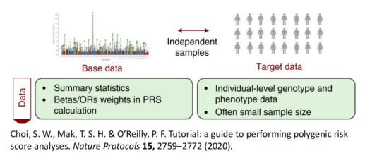
Choi, S. W., Mak, T. S. H. & O’Reilly, P. F. Tutorial: a guide to performing polygenic risk score analyses. Nature Protocols 15, 2759–2772 (2020).

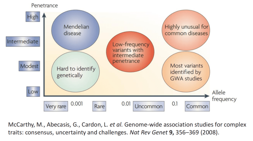
McCarthy, M., Abecasis, G., Cardon, L. et al. Genome-wide association studies for complex traits: consensus, uncertainty and challenges. Nat Rev Genet 9, 356–369 (2008).

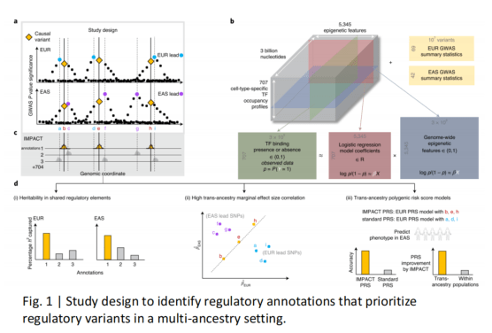
Amariuta, T. et al. Improving the trans-ancestry portability of polygenic risk scores by prioritizing variants in predicted cell-typespecific regulatory elements. Nature Genetics 52, 1346–1354 (2020).

使用GWAS概括性数据进行条件分析 GCTA – COJO

GCTA-COJO: multi-SNP-based conditional & joint association analysis using GWAS summary data

本文内容：

背景介绍
GCTA-COJO使用方法
参考样本的选择
参考

背景介绍：

通常情况下GWAS或是meta分析检验的是基于单个SNP模型的相关，所估计的效应量为被检验SNP的边际效应，但相比于多SNP模型的联合效应，单个SNP模型的边际效应并没有考虑该SNP与周围SNP的LD。

这会带来两个问题：

如果两个SNP成负相关，那么这两个SNP的效应都会被减弱。
如果两个SNP都达到了显著的阈值，事后很难通过LD来确定这两个SNP的相关的程度。

如果我们有原始样本层面的基因型，以及单SNP检验后的概括性数据，就可以在没有表型数据的情况下，将边缘效应转化为联合效应。

但一般情况下，对于一个包含很多队列的meta分析，我们无法获取个体的基因型数据，所以不能计算X′X（转化为联合效应时必须的步骤），但X′X本质上是一个SNP基因型的协方差矩阵，我们可以通过1.meta-analysis的基因型频率，与2.从可以获得基因型的参考样本计算而得的SNP之间的LD，来进行估计。这样的基于meta分析的基因频率与参考队列的LD的估计过程也可以用在相应的条件分析之中。（详细推导过程见原文）

使用方法：

COJO内置于GCTA软件中：

输入文件为

来自meta分析的概括性数据 summary-level statistics from a meta-analysis GWAS
参考样本的基因组文件 plink格式

-cojo-file [test.ma](<http://test.ma/>) 用于指定概括性数据：

概括性数据输入文件格式如下所示，

SNP A1 A2 freq b se p N 
rs1001 A G 0.8493 0.0024 0.0055 0.6653 129850 
rs1002 C G 0.0306 0.0034 0.0115 0.7659 129799 
rs1003 A C 0.5128 0.0045 0.0038 0.2319 129830
...

需要包含，各列需要按次顺序排列，列名则没有要求

1.SNP的ID，
2.效应等位A1，      #注意 A1,A2不能颠倒
3.参考等位A2，
4.效应等位的频率，   #也就是A1的频率
5.效应的大小，
6.标准差，
7.p值，
8.以及样本大小

注意

1.对于病例对照研究，效应大小应当是 log(odds ratio),以及其相对应的标准差。

即使你的研究对象只是一部分SNP，在准备输入文件时，也要准备所有SNP的概括性数据，主要原因是GCTA-COJO需要所有SNP的概括性数据来计算表型方差。可以使用--extract选项来限制COJO分析的区域。

COJO分析中可用的选项：

--cojo-slct

通过逐步法筛选出独立关联的SNP。结果将保存在*.jma文件中，还会有一个额外的文件*.jma.ldr保存SNP两两间的LD。

--cojo-top-SNPs 10

通过逐步法筛选出指定数量的独立关联的SNP，不设P值得阈值，找到指定数量的SNP为止。输出文件同--cojo-slct

--cojo-joint

不进行模型筛选，直接估计所有纳入的SNP的联合效应。输出文件同上。

--cojo-cond cond.snplist

校正给定列表中的SNP后进行关联分析。结果将保存在*.cma文件中。

其中cond.snplist的格式如下所示：

rs1001
rs1002
...

--cojo-p 5e-8

基因组范围显著的阈值，默认为 5e-8 。当使用–cojo-slct时，该选项才有效。

-cojo-wind 10000

当两个SNP的距离超过指定值时，认为其为连锁平衡的。默认值为10000 Kb (i.e. 10 Mb)

-cojo-collinear 0.9

模型选择时，程序会检查SNP之间的共线性问题，如果某一SNP在回归中的R2大于阈值，那么该SNP将不会被选择。默认值为0.9 。

-diff-freq 0.2

检查GWAS概括性数据中频率与参考样本中频率的差值，差值过大的SNP会被去除。默认值为0.2.

-cojo-gc

选择后p值会进行基因组控制。 e.g. –cojo-gc 1.05.

COJO分析的使用例：

# Select multiple associated SNPs through a stepwise selection procedure
gcta64  --bfile test  --chr 1 --maf 0.01 --cojo-file test.ma --cojo-slct --out test_chr1

# Select a fixed number of of top associated SNPs through a stepwise selection procedure
gcta64  --bfile test  --chr 1 --maf 0.01 --cojo-file test.ma --cojo-top-SNPs 10 --out test_chr1

# Estimate the joint effects of a subset of SNPs (given in the file test.snplist) without model selection
gcta64  --bfile test  --chr 1 --extract test.snplist  --cojo-file test.ma --cojo-joint --out test_chr1

# Perform single-SNP association analyses conditional on a set of SNPs (given in the file cond.snplist) without model selection
gcta64  --bfile test  --chr 1 --maf 0.01 --cojo-file test.ma --cojo-cond cond.snplist --out test_chr1

输出文件格式

结尾为.jma的文件（使用-cojo-slct 或 –cojo-joint时的输出）

Chr SNP bp freq refA b se p n freq_geno bJ bJ_se pJ LD_r
1 rs2001 172585028 0.6105 A 0.0377 0.0042 6.38e-19 121056 0.614 0.0379 0.0042 1.74e-19 -0.345
1 rs2002 174763990 0.4294 C 0.0287 0.0041 3.65e-12 124061 0.418 0.0289 0.0041 1.58e-12 0.012
1 rs2003 196696685 0.5863 T 0.0237 0.0042 1.38e-08 116314 0.589 0.0237 0.0042 1.67e-08 0.0 
...

输出文件的列依次是染色体号，SNP ID，位置，效应等位的频率，效应量大小，标准差，原始P值，估计的有效样本量，参考样本中的频率，joint analysis中该SNP的效应量大小，标准差，P值，以及列表中第i个SNP与第i+1个SNP的LD。

LD矩阵（使用-cojo-slct 或 –cojo-joint时的输出）

存储于后缀为jma.ldr的文件中

SNP rs2001 rs2002 rs2003 ...
rs2001 1 0.0525 -0.0672 ...
rs2002 0.0525 1 0.0045 ...
rs2003 -0.0672 0.0045 1 ...
...

结尾为.cma的文件（使用–cojo-cond选项会生成）

Chr SNP bp freq refA b se p n freq_geno bC bC_se pC
1 rs2001 172585028 0.6105 A 0.0377 0.0042 6.38e-19 121056 0.614 0.0379 0.0042 1.74e-19
1 rs2002 174763990 0.4294 C 0.0287 0.0041 3.65e-12 124061 0.418 0.0289 0.0041 1.58e-12
1 rs2003 196696685 0.5863 T 0.0237 0.0042 1.38e-08 116314 0.589 0.0237 0.0042 1.67e-08
...

GCTA-COJO 分析中参考样本的选择（重要！）

如果你的概括性数据来自单一的GWAS，那么最好的参考样本就是这个GWAS中的样本。
当概括性数据来自Meta分析，个体的基因型无法获取时，可以使用一个样本量较大队列的数据。例如，Wood et al. 2014 Nat Genet 使用了ARIC cohort (data available from dbGaP)
建议使用样本量大于4000的参考样本
不建议使用 HapMap 或 1000G 的参考样本，因为其样本量太小。

实际使用中可以使用填补后的基因型数据来估计LD，例如可以从BBJ中随机抽取20000个无关联的个体，提取其填补后的基因型作为EAS群体的参考面板。

参考：

Conditional and joint analysis method: Yang et al. (2012) Conditional and joint multiple-SNP analysis of GWAS summary statistics identifies additional variants influencing complex traits. Nat Genet 44(4):369-375. [PubMed ID: 22426310]

GCTA software: Yang J, Lee SH, Goddard ME and Visscher PM. GCTA: a tool for Genome-wide Complex Trait Analysis. Am J Hum Genet. 2011 Jan 88(1): 76-82. [PubMed ID: 21167468]

Eagle2单倍型定相工具 Haplotype phasing

本文内容：

 eagle2简介
 下载与安装
 使用方法
  无参考面板phasing
  有参考面板phasing
 输出
 附录：eagle -h
 参考

1.eagle2简介

Eagle是一款可在有参考面板或无参考面板的情况下，对样本的单倍体型进行估计的软件。 Eagle2目前是 Sanger 及Michigan 填充服务器的默认方法。该软件使用了一种快速的基于隐马尔科夫模型（HMM）的算法，大幅提升了速度与准确度。该软件的两个关键点为：基于 Burrows-Wheeler transform的一种新的数据结构，以及只探索HMM最相关路径的快速搜索算法。

2.下载与安装：

下载地址：http://data.broadinstitute.org/alkesgroup/Eagle/downloads/

文档地址：https://alkesgroup.broadinstitute.org/Eagle/Eagle_manual.html#x1-30002

平台要求：LINUX

内存要求：

无参考panel时，内存占用与样本数N以及SNP数呈线性关系。例如：UKBB 150K的样本，每1000个SNP需要1GB 内存。

有参考panel时，每个基因型需要约1.5个字节。

3 基本使用方法

下载安装后可以直接使用，选项可由以下格式指定 --optionName=optionValue.

一个最简单的示例如下：

./eagle --bfile=plink --geneticMapFile=USE_BIM --outPrefix=phased

eagle支持多线程，可以使用--numThreads来指定eagle使用的CPU核心数。

4.1 无参考面板的Phasing

1.输入

使用-bfile=prefix 指定输入的PLINK文件，注意eagle一次只phase一条染色体，如果PLINK文件里包含多条染色体，则需要通过-chrom指定染色体。

注意： PLINK在表示chr X （chrom 23=X）的non-PAR部分时，将所有男性的未丢失的基因型都转换为纯合，在表示PAR1与PAR2时（chrom 25=XY），则使用一般的二倍体基因型。如果只是想对chr X 的non-PAR部分进行phasing，那么只需输入 chrom 23 即可。如果要对整个X染色体（包括PAR与non-PAR），那么需要首先将plink文件中PAR与non-PAR的基因型合并，（可以使用plink的-merge-x）。VCF文件则不需要额外处理。

2.参考的遗传图谱

如果你的PILNK文件没有相应的遗传坐标文件（单位为摩根），可以使用eagle提供的事先处理好的参考图谱（从HapMap下载并转换格式）。使用时，选项如下：

-geneticMapFile=tables/genetic_map_hg##_withX.txt.gz

3.缺失值处理

phasing过程中，缺失的基因型会被自动填补。eagle输出的是best-guess单倍体基因型。如果不需要自动填补，输入文件为VCF,BCF时，则可以使用 --noImpMissing 来禁用自动填补功能。

4.基因型QC

当使用PLINK文件时，eagle会根据丢失率自动对样本与SNP进行QC，默认的阈值为0.01（自动去掉丢失率高于1%的样本或SNP）. eagle也可以通过指定–maxMissingPerSnp 与 –maxMissingPerIndiv 来手动对样本与SNP进行QC，但通常我们会使用QC过得PLINK文件，所以这一步可以使用–maxMissingPerSnp 1 与 –maxMissingPerIndiv 1（允许的最大丢失率为1，也就是没有施加任何QC）来略过这一步。在使用VCF文件时，eagle则不进行任何QC

5.样本与SNP的过滤

输入使用plink文件时，可以通过 –remove 与 –exclude 来对样本与SNP进行过滤

对于PLINK与VCF/BCF输入，可以使用 –bpStart and –bpEnd来限定phasing的区域（例如： –bpStart=50e6 以及–bpEnd=100e6）

6.模型参数指定

eagle2中主要调节运算速度与准确度平衡的参数选项为 –Kpbwt，该参数指定在各个样本的phasing中eagle2使用的调节单倍体型的数量，默认值为10000.

使用例：

./eagle \
	--bfile=plink_hg19 \
	--geneticMapFile=genetic_map_hg19_withX.txt.gz \
	--chrom=1 \
	--outPrefix=phased \
	--maxMissingPerSnp=1 \
	--maxMissingPerIndiv=1 \
	--numThreads=8

4.2 有参考面板Phasing

注意如果你的样本量是参考面板样本量的两倍以上时，使用参考样本并不会大幅提升phasing的精度。使用参考面板时，输入只能是VCF或BCF格式，分别使用–vcfTarget and –vcfRef 里指定目标以及参考样本的经过tabix索引的vcf，bcf文件。

如果vcf，bcf文件中含有多条染色体的数据，那么需要用–chrom 来指定。

其余的选项与无参考时vcf输入的情况支持的选项相似。

参考面板可以使用1000 genome的数据，但须经过一定处理，详见：https://alkesgroup.broadinstitute.org/Eagle/ 中5.3 Reference panels from the 1000 Genomes Project

5 输出

当输入为PLINK文件时，eagle输出为gzip压缩后的Oxford HAPS/SAMPLE 格式文件（详见SHAPEIT2 ），输出文件前缀可由–outPrefix 指定。

当输入为VCF，BCF文件时，输出也出VCF，BCF文件。输出文件前缀可由–outPrefix 指定。可用 –vcfOutFormat=z 指定输出文件格式。

6 附录

./eagle -h
                      +-----------------------------+
                      |                             |
                      |   Eagle v2.4.1              |
                      |   November 18, 2018         |
                      |   Po-Ru Loh                 |
                      |                             |
                      +-----------------------------+

Copyright (C) 2015-2018 Harvard University.
Distributed under the GNU GPLv3+ open source license.

Command line options:

eagle -h 

Options:

  --geneticMapFile arg             HapMap genetic map provided with download: 
                                   tables/genetic_map_hg##.txt.gz
  --outPrefix arg                  prefix for output files
  --numThreads arg (=1)            number of computational threads

Input options for phasing without a reference:
  --bfile arg                      prefix of PLINK .fam, .bim, .bed files
  --bfilegz arg                    prefix of PLINK .fam.gz, .bim.gz, .bed.gz 
                                   files
  --fam arg                        PLINK .fam file (note: file names ending in 
                                   .gz are auto-decompressed)
  --bim arg                        PLINK .bim file
  --bed arg                        PLINK .bed file
  --vcf arg                        [compressed] VCF/BCF file containing input 
                                   genotypes
  --remove arg                     file(s) listing individuals to ignore (no 
                                   header; FID IID must be first two columns)
  --exclude arg                    file(s) listing SNPs to ignore (no header; 
                                   SNP ID must be first column)
  --maxMissingPerSnp arg (=0.1)    QC filter: max missing rate per SNP
  --maxMissingPerIndiv arg (=0.1)  QC filter: max missing rate per person

Input/output options for phasing using a reference panel:
  --vcfRef arg                     tabix-indexed [compressed] VCF/BCF file for 
                                   reference haplotypes
  --vcfTarget arg                  tabix-indexed [compressed] VCF/BCF file for 
                                   target genotypes
  --vcfOutFormat arg (=.)          b|u|z|v: compressed BCF (b), uncomp BCF (u),
                                   compressed VCF (z), uncomp VCF (v)
  --noImpMissing                   disable imputation of missing target 
                                   genotypes (. or ./.)
  --allowRefAltSwap                allow swapping of REF/ALT in target vs. ref 
                                   VCF
  --outputUnphased                 output unphased sites (target-only, 
                                   multi-allelic, etc.)
  --keepMissingPloidyX             assume missing genotypes have correct ploidy
                                   (.=haploid, ./.=diploid)
  --vcfExclude arg                 tabix-indexed [compressed] VCF/BCF file 
                                   containing variants to exclude from phasing

Region selection options:
  --chrom arg (=0)                 chromosome to analyze (if input has many)
  --bpStart arg (=0)               minimum base pair position to analyze
  --bpEnd arg (=1e9)               maximum base pair position to analyze
  --bpFlanking arg (=0)            (ref-mode only) flanking region to use 
                                   during phasing but discard in output

Algorithm options:
  --Kpbwt arg (=10000)             number of conditioning haplotypes
  --pbwtIters arg (=0)             number of PBWT phasing iterations (0=auto)
  --expectIBDcM arg (=2.0)         expected length of haplotype copying (cM)
  --histFactor arg (=0)            history length multiplier (0=auto)
  --genoErrProb arg (=0.003)       estimated genotype error probability
  --pbwtOnly                       in non-ref mode, use only PBWT iters 
                                   (automatic for sequence data)
  --v1                             use Eagle1 phasing algorithm (instead of 
                                   default Eagle2 algorithm)

7 参考：

https://alkesgroup.broadinstitute.org/Eagle/

Loh P-R, Danecek P, Palamara PF, Fuchsberger C, Reshef YA, Finucane HK, Schoenherr S, Forer L, McCarthy S, Abecasis GR, Durbin R, and Price AL. Reference-based phasing using the Haplotype Reference Consortium panel. Nature Genetics (2016).

SNP的rsID与位置信息的相互匹配 rsID/ chr:pos conversion

本文内容：

1 个别SNP位点或rsID查询 
	dbsnp网页查询
2 少量转换可用的网页工具 （100,000 snp以内）
	SNP-nexus网页工具 
	vep注释工具网页版
3 大量转换使用的命令行工具 
	ANNOVAR命令行
	VEP命令行
4 参考

rsID与染色体位置信息的匹配或转换是生物信息学研究中必不可少的，但却又是十分繁琐的一项步骤，很多同学都在纠结这个问题，本文将总结常用的转换方法，以供参考：

转换前需要考虑的问题：

变异的标准化：Variant Normalization 变异的标准化
参考基因组的版本：人类参考基因组 Human reference genome hg19/hg38/GRCh37/GRCh38/b37/hs375d

1.个别SNP的转换：

直接使用dbsnp（详见：SNP数据库 – dbSNP）查询，查询个别SNP时方便快捷，可以直接搜rsID

也可以以chr:pos的形式搜rsID

2.少量转换可用的网页工具（100,000 snp以内）

2.1 SNPnexus : https://www.snp-nexus.org/v4/

首先输入用户信息，学术用途是免费的，使用自己的edu邮箱即可

之后选择assembly的版本

选择后可以通过多种方式提交自己要查询的SNP

2.1.1 这里我们通过上传文件的方式对rsID进行注释

输入文件 snp.txt 格式如下（其他格式的具体描述详见：https://www.snp-nexus.org/v4/guide/）

dbsnp   rs293794
dbsnp   rs1052133
dbsnp   rs3136820
dbsnp   rs2272615
dbsnp   rs2953993
dbsnp   rs1799782
dbsnp   rs25487
dbsnp   rs2248690
dbsnp   rs4918
dbsnp   rs1071592

然后是注释用的数据选择，各数据库版本见：https://www.snp-nexus.org/v4/guide/#data_source

因为我们只查询位置信息，就不勾选其他数据库，只使用默认的Ensembl

点击submit query后，稍作等待，结果就会显示出来，可以导出为VCF或txt文本格式。

2.1.2 位点转换为rsID时，输入文件如下：

格式为：< Type Name Position Allele1 Allele2 Strand > # Genomic position data for novel SNPs

chromosome	1	9262273	G	A	1
chromosome	1	45015006	G	A	1
chromosome	1	226982947	C	T	1
chromosome	2	189001450	G	A	1
chromosome	17	46010375	T	C	1

提交后即可查询，结果如下所示

2.2 VEP网页版

VEP注释工具使用详见（预留链接）

VEP网页版：https://asia.ensembl.org/info/docs/tools/vep/online/index.html

点击launch VEP

2.2.1 可以在input data处直接粘贴要查询的rsID，或是上传文件

点击输入框下方的example，可以查看可用的输入格式

这里以Variant identifiers 为例：

选择合适数据库，提交后可以看到查询状态

完成后点击View results

可查看基本信息，也可以导出

2.2.2 位点转换rsID时，使用如下Ensembl默认的输入格式即可：

3.大量转换时的命令行工具

3.1 可使用如上所述VEP工具的命令行版本

下载地址与文档见：https://asia.ensembl.org/info/docs/tools/vep/index.html

3.2 也可以使用ANNOVAR

安装与使用具体使用方法见：使用ANNOVAR 对Variants进行功能注释 Annotation POST-GWAS analysis

这里只简单介绍rsID与chr：pos互相转换的方法

3.2.1 rsID转chr：pos

使用ANNOVAR的convert2annovar.pl 程序与-format rsid选项即可注释位置信息，使用例如下所示，

（注意参考基因组的版本）

[kaiwang@biocluster ~/]$ cat example/snplist.txt 
rs74487784
rs41534544
rs4308095
rs12345678

[kaiwang@biocluster ~/]$ convert2annovar.pl -format rsid example/snplist.txt -dbsnpfile humandb/hg19_snp138.txt > snplist.avinput 
NOTICE: Scanning dbSNP file humandb/hg19_snp138.txt...
NOTICE: input file contains 4 rs identifiers, output file contains information for 4 rs identifiers
WARNING: 1 rs identifiers have multiple records (due to multiple mapping) and they are all written to output

[kaiwang@biocluster ~/]$ cat snplist.avinput 
chr2 186229004 186229004 C T rs4308095
chr7 6026775 6026775 T C rs41534544
chr7 6777183 6777183 G A rs41534544
chr9 3901666 3901666 T C rs12345678
chr22 24325095 24325095 A G rs74487784

3.2.2 chr：pos转rsID

位点信息转化为rsID时需要使用基于筛选的注释：

这里使用avsnp150，具体描述可见：https://annovar.openbioinformatics.org/en/latest/user-guide/download/

使用方法如下：

#首先下载注释用数据库：
annotate_variation.pl -downdb -webfrom annovar -buildver hg19 avsnp150 humandb/

#完成后即可进行转换
annotate_variation.pl ex1.avinput humandb/ -filter -build hg19 -dbtype avsnp150

输入文件使用上述的（类bed文件），ex1.avinput

chr2 186229004 186229004 C T
chr7 6026775 6026775 T C
chr7 6777183 6777183 G A
chr9 3901666 3901666 T C
chr22 24325095 24325095 A G

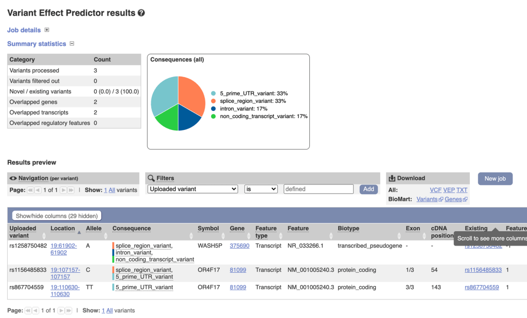
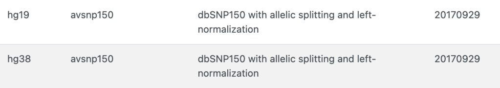
输出文件如下，ex1.avinput.hg19_avsnp150_dropped，

（注意某些SNP的rsID有合并等原因，版本不同rsID注释结果不一定相同）

avsnp150        rs4308095       chr2 186229004 186229004 C T
avsnp150        rs140195        chr22 24325095 24325095 A G
avsnp150        rs2228006       chr7 6026775 6026775 T C
avsnp150        rs766725467     chr7 6777183 6777183 G A
avsnp150        rs12345678      chr9 3901666 3901666 T C

注释rsID可能会遇到的问题：

https://annovar.openbioinformatics.org/en/latest/articles/dbSNP/

参考：

dbsnp：https://www.ncbi.nlm.nih.gov/snp/

annovar：https://annovar.openbioinformatics.org/en/latest/

vep：https://asia.ensembl.org/info/docs/tools/vep/index.html

snpnexus：https://www.snp-nexus.org/v4/

GWAS方法 – SAIGE 校正样本对照失衡的广义线性混合模型

关键词：saige，GLMM，case-control imbalance，binary phenotype， SPA

本文内容：

SAIGE开发背景
SAIGE原理简介
	第一步
	第二步
	注意事项
SAIGE使用方法
	安装
	第一步
	第二步
	结果解读
参考

一句话解释：SAIGE是一种基于广义线性混合模型的，针对二分类表型（binary phenotype）能够调整样本对照不平衡（case-control imbalance）与隐性关联（cryptic relatedness）的GWAS检验方法。

① SAIGE开发背景：

在大规模生物银行，对上千种表型进行的GWAS中，大多数二分类变量的病例都远小于对照，线性混合模型，或逻辑斯蒂混合模型对于此种病例对照严重失衡（1:10，甚至到1:100）的表型，都不能很好地控制1类错误，容易造成假阳性出现。

SAIGE便是针对此问题开发的方法，目前UKBB等GWAS概括性数据所使用的方法均为SAIGE。SAIGE的特点是利用 SPA（saddlepoint approximation ，鞍点近似法）在病例对照比例严重失衡时，仍然获得准确的p值。

② SAIGE原理简介：

SAIGE全称是 Scalable and Accurate Implementation of GEneralized mixed model 广义混合模型的可扩展且准确的实现。

SAIGE 与 bolt-lmm 或 regenie 类似，都需要两个步骤。saige基于广义线性混合模型GLMM模型：

https://gwaslab.org/wp-content/uploads/2021/04/image-26.png?w=301

其中

为给定协变量与基因型时，第i个样本为病例的概率，bi为随机效应，服从N(0，τψ)的分布。其中ψ是N X N的遗传关联矩阵（GRM），τ是加性遗传方差。Xi为协变量，Gi表示等位基因的个数，取值为0,1，2，α为（1+p）x 1 的表示固定效应的系数向量，β为遗传效应的系数。

具体流程如下：

第一步（构建null模型），估计方差与其他参数：

利用 array genotype ，估计 null 逻辑斯蒂混合模型（GLMM）。

https://gwaslab.org/wp-content/uploads/2021/04/image-27.png?w=236

SAIGE通过PQL方法和 AI-REML 算法简化计算提高效率。

迭代估计模型中参数：

每一次迭代中，让

为y的估计的均值，

则权重矩阵为

让

为N X N的如下工作向量的方差矩阵

目前诸如GMMAT等方法在这一步时需要计算该方差矩阵的逆，

当N较大时，该步骤计算量巨大，为了简化计算，SAIGE采用了PCG算法（PCG是一种找到线性系统解的数值方法，BOLT_LMM也用到此算法）

在如下零假设（null hypothesis）的情况下：

分数检验统计量由下式得到

其方差Var（T）为

其中

因为我们需要对每一个SNP都计算P，计算量巨大，

SAIGE假设真随机效应b已经给定，并计算两种情况下T的方差的比值，来进行简化计算。

假设b给定时：

则方差比值r

saige中会取随机取30个snp来估计r。

第二步（检验）：分数检验，并通过SPA调整。

采用上述比值r对分数检验的T检验量进行调整，即可得到SAIGE的T检验量。

一般情况下，传统方法假设T渐进服从一个高斯分布，但是当病例对照（case-control）的比例不平衡，以及被检验变异有较低的MAC（Minor allele count）时，T统计量就会与高斯分布有显著偏离。saige方法之所以能调节病例对照不平衡，关键点就在于利用SPA对检验的调整，以获得一个较为准确的P值。（saige采用了fastSPA）

SPA：saddlepoint approximation (SPA) 鞍点近似法

SAIGE整体架构如下所示：

https://github.com/weizhouUMICH/img/raw/master/SAIGE2step.png

③ SAIGE的注意事项：

注意：该比值只有在MAC大于30时，才保持恒定，当MAC小于30时，要谨慎使用此方法

④ SAIGE使用方法：

saige的github页面：https://github.com/weizhouUMICH/SAIGE

安装：

saige是基于R的软件，有多种安装方法：

可以通过R安装，也可以通过CONDA安装，但安装过程复杂，个人推荐使用docker进行安装，方便快捷。

docker pull wzhou88/saige:0.44.2

第一步，估计空模型

输入文件：

1 基因型文件PLINK格式

2 表性文件

3 协变量文件

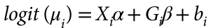
#For Binary traits:
Rscript step1_fitNULLGLMM.R     \
        --plinkFile=./input/nfam_100_nindep_0_step1_includeMoreRareVariants_poly \
        --phenoFile=./input/pheno_1000samples.txt_withdosages_withBothTraitTypes.txt \
        --phenoCol=y_binary \
        --covarColList=x1,x2 \
        --sampleIDColinphenoFile=IID \
        --traitType=binary        \
        --outputPrefix=./output/example_binary \
        --nThreads=4 \
        --LOCO=FALSE \
        --IsOverwriteVarianceRatioFile ## v0.38. Whether to overwrite the variance ratio file if the file already exists

#For Quantitative traits, if not normally distributed, inverse normalization needs to be specified to be TRUE --invNormalize=TRUE
Rscript step1_fitNULLGLMM.R     \
        --plinkFile=./input/nfam_100_nindep_0_step1_includeMoreRareVariants_poly \
        --phenoFile=./input/pheno_1000samples.txt_withdosages_withBothTraitTypes.txt \
        --phenoCol=y_quantitative \
        --covarColList=x1,x2 \
        --sampleIDColinphenoFile=IID \
        --traitType=quantitative       \
		--invNormalize=TRUE	\
        --outputPrefix=./output/example_quantitative \
        --nThreads=4 \\
        --LOCO=FALSE	\\
	--tauInit=1,0

共有三个输出文件：

.rda文件，包含空模型
30个随机选择的SNP的关联结果
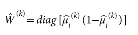
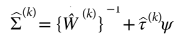
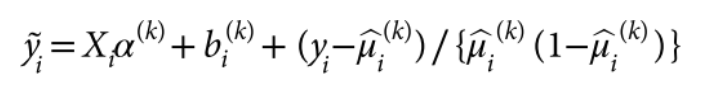
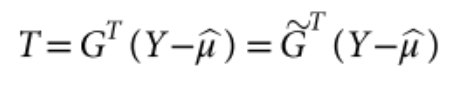
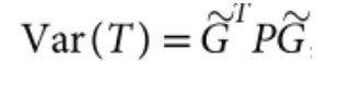
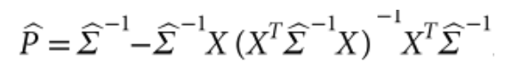
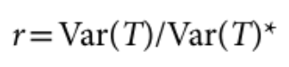
包含估计的方差比值的文本文件（回忆上述SAIGE算法中的r

.rda文件，包含空模型

./output/example_quantitative.rda

#open R
R
#load the model file in R
load("./output/example_quantitative.rda")
names(modglmm)
modglmm$theta

#theta: a vector of length 2. The first element is the dispersion parameter estimate and the second one is the variance component parameter estimate
#coefficients: fixed effect parameter estimates
#linear.predictors: a vector of length N (N is the sample size) containing linear predictors
#fitted.values: a vector of length N (N is the sample size) containing fitted mean values on the original scale
#Y: a vector of length N (N is the sample size) containing final working vector
#residuals: a vector of length N (N is the sample size) containing residuals on the original scale
#sampleID: a vector of length N (N is the sample size) containing sample IDs used to fit the null model

30个随机选择的SNP的关联结果

less -S ./output/example_quantitative_30markers.SAIGE.results.txt

方差比值文件 variance ratio file

less -S ./output/example_quantitative.varianceRatio.txt

第二步

输入文件为：

1 插补后的剂量文件，如VCF，BGEN，BCF或SAV，以及

2 对应的索引文件

3 样本文件，无header，包含一列对应剂量文件的样本ID。

4 第一步所得的rda模型文件

5 第一步所得的方差比值文件

这里以常用的bgen与VCF文件为例

#bgen for dosages
Rscript step2_SPAtests.R \
        --bgenFile=./input/genotype_100markers.bgen \
        --bgenFileIndex=./input/genotype_100markers.bgen.bgi \
        --minMAF=0.0001 \ #最小MAF不能低于0.0001
        --minMAC=1 \ #最小MAC不能低于1
        --sampleFile=./input/samplefileforbgen_10000samples.txt \
        --GMMATmodelFile=./output/example.rda \
        --varianceRatioFile=./output/example.varianceRatio.txt \
        --SAIGEOutputFile=./output/example.SAIGE.bgen.txt \
        --numLinesOutput=2 \
        --IsOutputAFinCaseCtrl=TRUE

#VCF containing dosages (--vcfField=DS)
Rscript step2_SPAtests.R \
        --vcfFile=./input/dosage_10markers.vcf.gz \
        --vcfFileIndex=./input/dosage_10markers.vcf.gz.tbi \
        --vcfField=DS \
        --chrom=1 \
        --minMAF=0.0001 \   #最小MAF不能低于0.0001
        --minMAC=1 \   #最小MAC不能低于1
        --sampleFile=./input/sampleIDindosage.txt \
        --GMMATmodelFile=./output/example.rda \
        --varianceRatioFile=./output/example.varianceRatio.txt \
        --SAIGEOutputFile=./output/example.SAIGE.vcf.dosage.txt \
        --numLinesOutput=2 \
        --IsOutputAFinCaseCtrl=TRUE

输出结果各列的解读如下：

CHR: chromosome
POS: genome position 
SNPID: variant ID
Allele1: allele 1
Allele2: allele 2
AC_Allele2: allele count of allele 2
AF_Allele2: allele frequency of allele 2
imputationInfo: imputation info. If not in dosage/genotype input file, will output 1
N: sample size
BETA: effect size of allele 2
SE: standard error of BETA
Tstat: score statistic of allele 2

#SPA后的p值
p.value: p value (with SPA applied for binary traits) 

p.value.NA: p value when SPA is not applied (only for binary traits)
Is.SPA.converge: whether SPA is converged or not (only for binary traits)
varT: estimated variance of score statistic with sample relatedness incorporated
varTstar: variance of score statistic without sample relatedness incorporated
AF.Cases: allele frequency of allele 2 in cases (only for binary traits and if --IsOutputAFinCaseCtrl=TRUE)
AF.Controls: allele frequency of allele 2 in controls (only for binary traits and if --IsOutputAFinCaseCtrl=TRUE)
Tstat_cond, p.value_cond, varT_cond, BETA_cond, SE_cond: summary stats for conditional analysis

除此之外SAIGE还支持条件分析，男女分层分析，X染色体分析等多种功能：

详细文档见：https://github.com/weizhouUMICH/SAIGE/wiki/Genetic-association-tests-using-SAIGE#installing-saige

参考：

Zhou, W. et al. (SAIGE)Efficiently controlling for case-control imbalance and sample relatedness in large-scale genetic association studies. Nat. Genet. 50, 1335–1341 (2018).

基因组控制与基因组膨胀系数λ Genomic control λGC

本文内容


什么是基因组控制 Genomic Control
基因组膨胀系数λGC （Genomic Inflation Factor） 的计算方法
GC的注意事项以及解决办法

什么是基因组控制 Genomic Control

基因组控制是矫正GWAS中因群体分层等原因而导致检验统计量膨胀的一种方法。

考虑一种简单病例对照研究，假设有N个样本，以及n个SNP，φ是样本中病例的比例(0<φ<1), 对于某个SNP，其在病例以及对照中的频率如下表所示：

为了检验关联性，我们会基于隐形，显性，以及加性遗传模型来计算自由度为1的卡方检验量。这里以加性遗传模型为例，对SNP进行趋势检验 ( Armitage’s trend test）。其计算公式为：

我们假设对于每个SNP，我们都计算了其相应的趋势检验的Y2l统计量，当这些SNP之间没有连锁不平衡LD，且不存在人群分层以及隐性关联时，检验量Y2服从卡方分布。

基因组控制（Genomic control，GC）模型假设是这些检验统计量会因为群体分层以及隐形关联等原因出现膨胀，膨胀系数为 λ （基因组膨胀系数 Genomic Inflation Factor）。同时GC模型假设这个膨胀系数在基因组上对于所有SNP是近似相等的。

2.基因组膨胀系数 Genomic Inflation Factor 的计算方法

基于此我们可以通过下式来估计λGC ，

取GWAS检验后所有卡方检验量的中间值，除以0.456，其中0.456为卡方检验量的期望值（卡方分布中，第50百分位数的卡方统计量，r语言中qchisq(0.5，1)对应的值）。之所以取中间值计算λGC是因为要避免异常值的影响。

λ越接近1，就表明不存在群体分层导致的统计量膨胀。

将GWAS检验后所有卡方统计量除以λ后重新计算p值得过程即为基因组控制 GC。

例如这个GWAS研究的QQ图，可以看到观测值有一个明显的系统性的抬升，这通常意味着样本中存在在群体分层，通过计算我们得到这个GWAS研究的基因组膨胀系数为 λ=1.17，

将原始的统计量除以1.17，重新计算p值后，可以看到之前的抬升得到有效控制。

3. GC的注意事项以及解决办法：

但要注意的是，GC假设基因组中只有少数的loci与表型相关，绝大多数被检验的SNP是与表型无关的，而目前的主流GWAS检验方法大多基于无限小模型（infinitesimal model）(详见：解释复杂疾病的四种主流模型 CDCV/RAME/infinitesimal/Broad-sense-heritability)，该模型假设所有SNP与表型都是有关的，只是效应量很小。这种情况下就不再适用GC。

其他解决人群分层等的办法包括：

严格的质控QC GWAS前的质控（QC） GWAS Quality control
通过LD score回归来判别统计量的膨胀是因为人群分层等外部影响，还是多基因遗传结构的影响。连锁不平衡分数回归 LD score regression
使用LMM模型（线性混合模型 – LMM Linear Mixed Model）并将PCA的主成分加入协变量。群体分层与主成分分析 Population structure & PCA

等等

参考：

Devlin, B. & Roeder, K. Genomic control for association studies. Biometrics 55, 997–1004 (1999).

Devlin, B. Genomic control, a new approach to genetic-based associationb studies. (2001).

Genebass 外显子组关联检验数据库

关键词：外显子组， pLOF，UKBB，rare variants， gene-based analysis

本文目录：

1.背景
2.Genebass介绍
3.使用方法
4.参考

1.背景

目前为止大规模的GWAS研究已经成功的发现了大量的与人类疾病或表型相关的常见变异，但对于稀有变异与疾病的关联，我们目前还没有系统性的探索。生物银行规模的外显子组测序给我们提供了宝贵的机会以探索基因以及稀有编码变异对于人类表性的影响。UKBB的主要研究人员（Neale lab）利用UKBB的28万多人的外显子组测序数据，通过单核苷酸检验，与基因检验系统性地分析了3700种数量与二分类表型，并将数据公开在Genebass数据库中。

2.Genebass介绍：

Genebass数据集包含了3817种表型的基于基因与基于单变异检验的概括性数据，该数据库的概括性数据基于UK Biobank 28万1852人的外显子组测序数据。

检验方法使用的是基于线性混合模型，并校正case-control比例的SAIGE-GENE（预留链接，最近挖的坑有点多），包括了以下三种检验统计量：