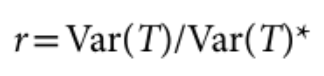
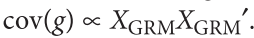
没有单独的研究有效样本量数据时可基于荟萃后的sumstats近似估计: 4/(2pq x SE^2). 其中pq为 MAF*(1-MAF)
详细推导和分析可以参考
Grotzinger, A. D., de la Fuente, J., Privé, F., Nivard, M. G., & Tucker-Drob, E. M. (2023). Pervasive downward bias in estimates of liability-scale heritability in genome-wide association study meta-analysis: a simple solution. Biological psychiatry, 93(1), 29-36.
与有效群体大小区别
有效群体大小 (Effective population size, Ne) 群体遗传学中一个重要的概念,其描述的是等效的理想化Wright–Fisher population群体的大小,决定了由genetic drift导致的群体构成发生的变化。其定义中的等效是对于某种遗传数值而言,可以指 allele variance (variance effective population size) 或 inbreeding coefficient (inbreeding effective population size)。概念上与有效样本量有类似之处,但具体所指对象不同,注意不要混淆。
Ziyatdinov, A., Kim, J., Prokopenko, D., Privé, F., Laporte, F., Loh, P. R., … & Aschard, H. (2021). Estimating the effective sample size in association studies of quantitative traits. G3, 11(6), jkab057.
参考
Grotzinger, A. D., de la Fuente, J., Privé, F., Nivard, M. G., & Tucker-Drob, E. M. (2023). Pervasive downward bias in estimates of liability-scale heritability in genome-wide association study meta-analysis: a simple solution. Biological psychiatry, 93(1), 29-36.
公式推导可以参考 Ghosh, A., Zou, F., & Wright, F. A. (2008). Estimating odds ratios in genome scans: an approximate conditional likelihood approach. The American Journal of Human Genetics, 82(5), 1064-1074. 中的Appendix A
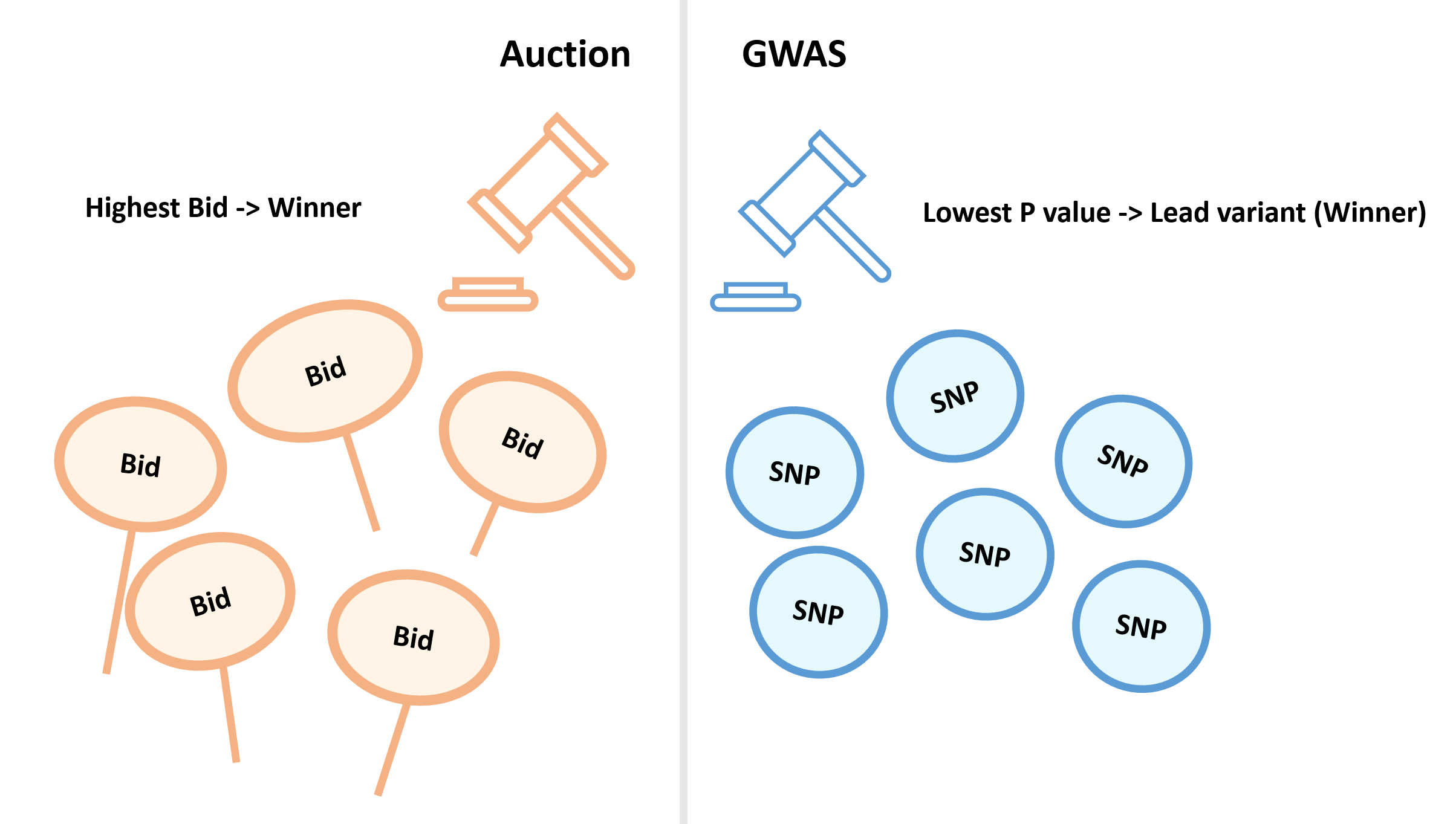
Bazerman, M. H., & Samuelson, W. F. (1983). I won the auction but don’t want the prize. Journal of conflict resolution, 27(4), 618-634.
Göring, H. H., Terwilliger, J. D., & Blangero, J. (2001). Large upward bias in estimation of locus-specific effects from genomewide scans. The American Journal of Human Genetics, 69(6), 1357-1369.
Zhong, H., & Prentice, R. L. (2008). Bias-reduced estimators and confidence intervals for odds ratios in genome-wide association studies. Biostatistics, 9(4), 621-634.
Ghosh, A., Zou, F., & Wright, F. A. (2008). Estimating odds ratios in genome scans: an approximate conditional likelihood approach. The American Journal of Human Genetics, 82(5), 1064-1074.
Skol, A. D., Scott, L. J., Abecasis, G. R., & Boehnke, M. (2006). Joint analysis is more efficient than replication-based analysis for two-stage genome-wide association studies. Nature genetics, 38(2), 209-213.
Johnson, J. L., & Abecasis, G. R. (2017). GAS Power Calculator: web-based power calculator for genetic association studies. BioRxiv, 164343.
Sham, P. C., & Purcell, S. M. (2014). Statistical power and significance testing in large-scale genetic studies. Nature Reviews Genetics, 15(5), 335-346.
head -n 20 tutorial_results_1.1NS.log
2021/10/31/10:43:32 PM
<><><<>><><><><><><><><><><><><><><><><><><><><><><><><><><><><><><><><><><>
<>
<> MTAG: Multi-trait Analysis of GWAS
<> Version: 1.0.8
<> (C) 2017 Omeed Maghzian, Raymond Walters, and Patrick Turley
<> Harvard University Department of Economics / Broad Institute of MIT and Harvard
<> GNU General Public License v3
<><><<>><><><><><><><><><><><><><><><><><><><><><><><><><><><><><><><><><><>
<> Note:  It is recommended to run your own QC on the input before using this program.
<> Software-related correspondence: maghzian@nber.org
<> All other correspondence: paturley@broadinstitute.org
<><><<>><><><><><><><><><><><><><><><><><><><><><><><><><><><><><><><><><><>

Calling ./mtag.py \
--stream-stdout  \
--n-min 0.0 \
--sumstats 1_OA2016_hm3samp_NEUR.txt,1_OA2016_hm3samp_SWB.txt \
--out ./tutorial_results_1.1NS
MTAG效应量估计值文件(trait_1):
head tutorial_results_1.1NS_trait_1.txt
SNP	CHR	BP	A1	A2	Z	N	FRQ	mtag_beta	mtag_se	mtag_z	mtag_pval
rs2736372	8	11106041	T	C	-7.7161416126199995	111111.11111099999	0.4179	-0.032488048690724455	0.004191057650619415	-7.751754186899077	9.063170638233748e-15
rs2060465	8	11162609	T	C	7.69444599845	62500.0	0.6194	0.038971244976047835	0.005364284755639267	7.264947099439278	3.731842884367329e-13
rs10096421	8	10831868	T	G	-7.561098219	111111.11111099999	0.4646	-0.0306226260844897350.004144573386350028	-7.388607518772383	1.483744201034853e-13
rs2409722	8	11039816	T	G	-7.382616018080001	111111.11111099999	0.4627	-0.032187004733709536	0.004145724613962613	-7.763903233057294	8.235474166666265e-15
rs11991118	8	10939273	T	G	7.32202915636	111111.11111099999	0.5056	0.030603923980300953 0.004134432028802615	7.402207550419989	1.339389362466671e-13
rs2736371	8	11105529	A	G	-7.32009158327	62500.0	0.3806	-0.03759068256663257	0.005364284755639268	-7.007585219467501	2.42466338629309e-12
rs2736313	8	11086942	T	C	-7.24228035161	111111.11111099999	0.4646	-0.03068115211425502 0.004144573386350028	-7.402728641577938	1.3341420385130596e-13
rs876954	8	8310923	A	G	-7.15791677597	62500.0	0.4813	-0.03422779585744538	0.005212736369758894 -6.566185862767606	5.162037825451834e-11
rs1533059	8	8684953	A	G	-7.074128564239999	62500.0	0.4478	-0.035027431607855014	0.00523771146606734	-6.687545091932079	2.269452965596589e-11
SNP A1 A2 freq b se p N
rs1001 A G 0.8493 0.0024 0.0055 0.6653 129850
rs1002 C G 0.0306 0.0034 0.0115 0.7659 129799
rs1003 A C 0.5128 0.0045 0.0038 0.2319 129830
...
# Select multiple associated SNPs through a stepwise selection procedure
gcta64  --bfile test  --chr 1 --maf 0.01 --cojo-file test.ma --cojo-slct --out test_chr1

# Select a fixed number of of top associated SNPs through a stepwise selection procedure
gcta64  --bfile test  --chr 1 --maf 0.01 --cojo-file test.ma --cojo-top-SNPs 10 --out test_chr1

# Estimate the joint effects of a subset of SNPs (given in the file test.snplist) without model selection
gcta64  --bfile test  --chr 1 --extract test.snplist  --cojo-file test.ma --cojo-joint --out test_chr1

# Perform single-SNP association analyses conditional on a set of SNPs (given in the file cond.snplist) without model selection
gcta64  --bfile test  --chr 1 --maf 0.01 --cojo-file test.ma --cojo-cond cond.snplist --out test_chr1
输出文件格式
结尾为.jma的文件 (使用-cojo-slct 或 –cojo-joint时的输出)
Chr SNP bp freq refA b se p n freq_geno bJ bJ_se pJ LD_r
1 rs2001 172585028 0.6105 A 0.0377 0.0042 6.38e-19 121056 0.614 0.0379 0.0042 1.74e-19 -0.345
1 rs2002 174763990 0.4294 C 0.0287 0.0041 3.65e-12 124061 0.418 0.0289 0.0041 1.58e-12 0.012
1 rs2003 196696685 0.5863 T 0.0237 0.0042 1.38e-08 116314 0.589 0.0237 0.0042 1.67e-08 0.0
...
Chr SNP bp freq refA b se p n freq_geno bC bC_se pC
1 rs2001 172585028 0.6105 A 0.0377 0.0042 6.38e-19 121056 0.614 0.0379 0.0042 1.74e-19
1 rs2002 174763990 0.4294 C 0.0287 0.0041 3.65e-12 124061 0.418 0.0289 0.0041 1.58e-12
1 rs2003 196696685 0.5863 T 0.0237 0.0042 1.38e-08 116314 0.589 0.0237 0.0042 1.67e-08
...
GCTA-COJO 分析中参考样本的选择(重要!)
如果你的概括性数据来自单一的GWAS,那么最好的参考样本就是这个GWAS中的样本。
当概括性数据来自Meta分析,个体的基因型无法获取时,可以使用一个样本量较大队列的数据。例如,Wood et al. 2014 Nat Genet 使用了ARIC cohort (data available from dbGaP)
Conditional and joint analysis method: Yang et al. (2012) Conditional and joint multiple-SNP analysis of GWAS summary statistics identifies additional variants influencing complex traits. Nat Genet 44(4):369-375. [PubMed ID: 22426310]
GCTA software: Yang J, Lee SH, Goddard ME and Visscher PM. GCTA: a tool for Genome-wide Complex Trait Analysis. Am J Hum Genet. 2011 Jan 88(1): 76-82. [PubMed ID: 21167468]
#For Binary traits:
Rscript step1_fitNULLGLMM.R     \
        --plinkFile=./input/nfam_100_nindep_0_step1_includeMoreRareVariants_poly \
        --phenoFile=./input/pheno_1000samples.txt_withdosages_withBothTraitTypes.txt \
        --phenoCol=y_binary \
        --covarColList=x1,x2 \
        --sampleIDColinphenoFile=IID \
        --traitType=binary        \
        --outputPrefix=./output/example_binary \
        --nThreads=4 \
        --LOCO=FALSE \
        --IsOverwriteVarianceRatioFile ## v0.38. Whether to overwrite the variance ratio file if the file already exists

#For Quantitative traits, if not normally distributed, inverse normalization needs to be specified to be TRUE --invNormalize=TRUE
Rscript step1_fitNULLGLMM.R     \
        --plinkFile=./input/nfam_100_nindep_0_step1_includeMoreRareVariants_poly \
        --phenoFile=./input/pheno_1000samples.txt_withdosages_withBothTraitTypes.txt \
        --phenoCol=y_quantitative \
        --covarColList=x1,x2 \
        --sampleIDColinphenoFile=IID \
        --traitType=quantitative       \
		--invNormalize=TRUE	\
        --outputPrefix=./output/example_quantitative \
        --nThreads=4 \\
        --LOCO=FALSE	\\
	--tauInit=1,0
共有三个输出文件:
.rda文件,包含空模型
30个随机选择的SNP的关联结果
包含估计的方差比值的文本文件 (回忆上述SAIGE算法中的r
.rda文件,包含空模型
./output/example_quantitative.rda

#open R
R
#load the model file in R
load("./output/example_quantitative.rda")
names(modglmm)
modglmm$theta

#theta: a vector of length 2. The first element is the dispersion parameter estimate and the second one is the variance component parameter estimate
#coefficients: fixed effect parameter estimates
#linear.predictors: a vector of length N (N is the sample size) containing linear predictors
#fitted.values: a vector of length N (N is the sample size) containing fitted mean values on the original scale
#Y: a vector of length N (N is the sample size) containing final working vector
#residuals: a vector of length N (N is the sample size) containing residuals on the original scale
#sampleID: a vector of length N (N is the sample size) containing sample IDs used to fit the null model
30个随机选择的SNP的关联结果
less -S ./output/example_quantitative_30markers.SAIGE.results.txt
方差比值文件 variance ratio file
less -S ./output/example_quantitative.varianceRatio.txt
CHR: chromosome
POS: genome position
SNPID: variant ID
Allele1: allele 1
Allele2: allele 2
AC_Allele2: allele count of allele 2
AF_Allele2: allele frequency of allele 2
imputationInfo: imputation info. If not in dosage/genotype input file, will output 1
N: sample size
BETA: effect size of allele 2
SE: standard error of BETA
Tstat: score statistic of allele 2

#SPA后的p值
p.value: p value (with SPA applied for binary traits)

p.value.NA: p value when SPA is not applied (only for binary traits)
Is.SPA.converge: whether SPA is converged or not (only for binary traits)
varT: estimated variance of score statistic with sample relatedness incorporated
varTstar: variance of score statistic without sample relatedness incorporated
AF.Cases: allele frequency of allele 2 in cases (only for binary traits and if --IsOutputAFinCaseCtrl=TRUE)
AF.Controls: allele frequency of allele 2 in controls (only for binary traits and if --IsOutputAFinCaseCtrl=TRUE)
Tstat_cond, p.value_cond, varT_cond, BETA_cond, SE_cond: summary stats for conditional analysis
Zhou, W. et al. (SAIGE)Efficiently controlling for case-control imbalance and sample relatedness in large-scale genetic association studies. Nat. Genet. 50, 1335–1341 (2018).
Jiang L, Zheng Z, Qi T, et al. A resource-efficient tool for mixed model association analysis of large-scale data[J]. Nature genetics, 2019, 51(12): 1749-1755.
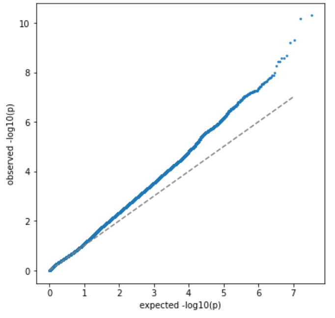
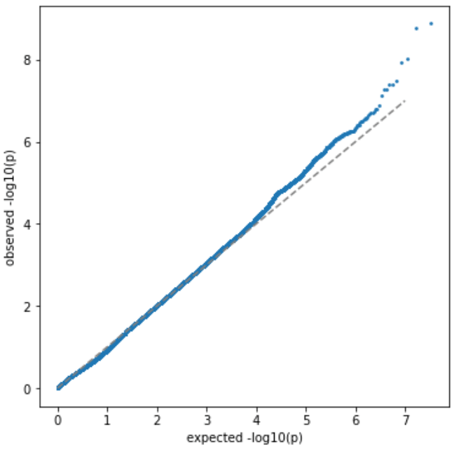
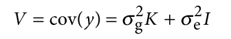
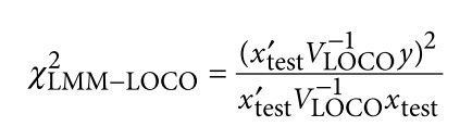
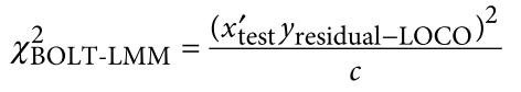
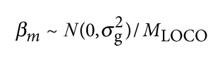
为了避免此现象造成的power损失,理论上在构建null模型中排除掉待检验SNP是正确的做法,但这样太占运算资源,所以在实践中,我们会采用 LOCO Leave-one-chromosome-out ,即使用排除掉待检验SNP所在的染色体的所有SNP,再进行检验(也就是说我们有对应22个常染色体的loco null模型)。


 的近似分布为:
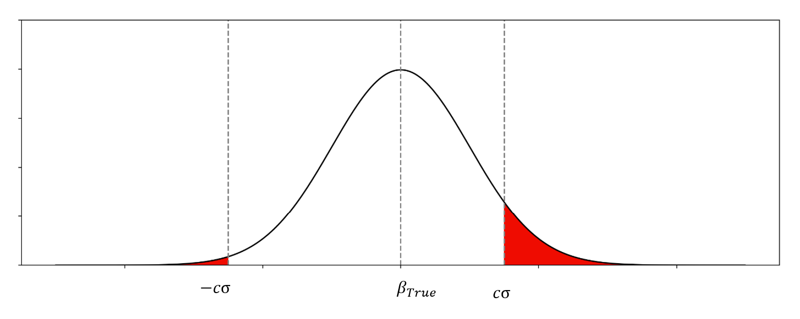

 的一个例子
的一个例子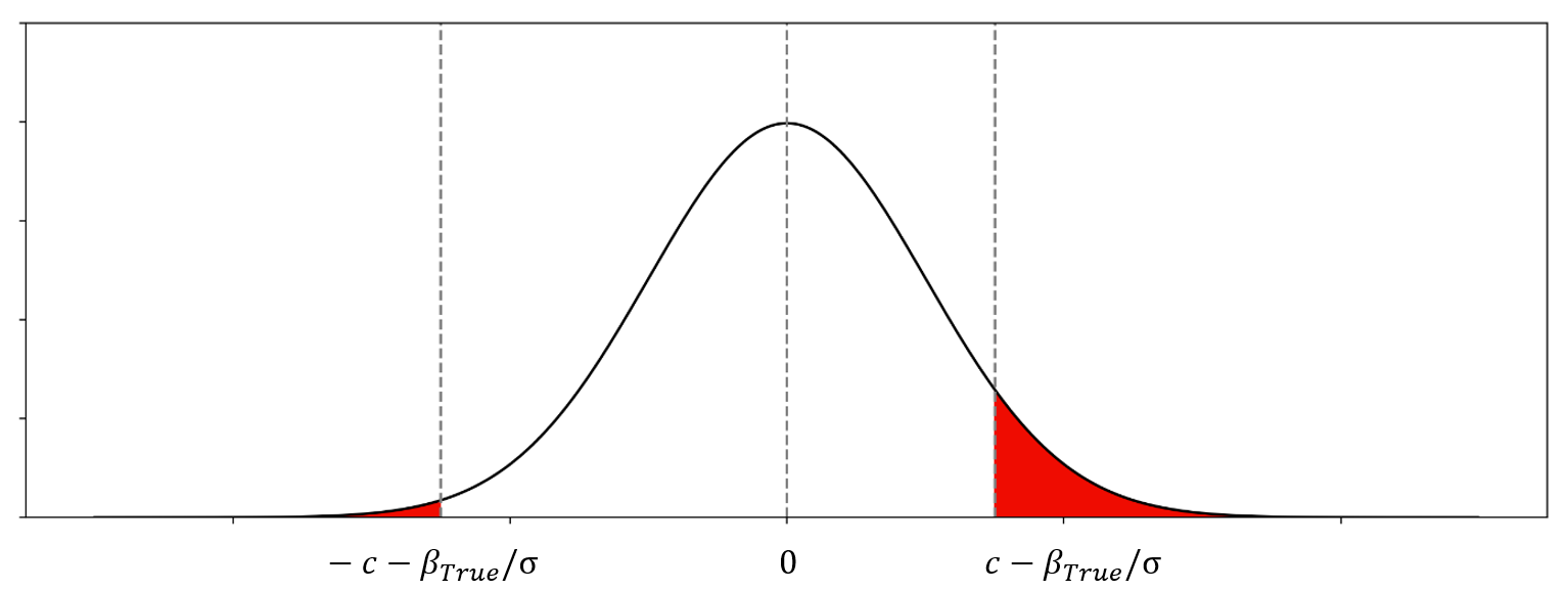


 : 标准正态分布的概率密度函数
 : 标准正态分布的累积分布函数
 , SE
, SE  , 以及用于筛选的显著性阈值决定.
 与统计学检验结果(是否拒绝原假设


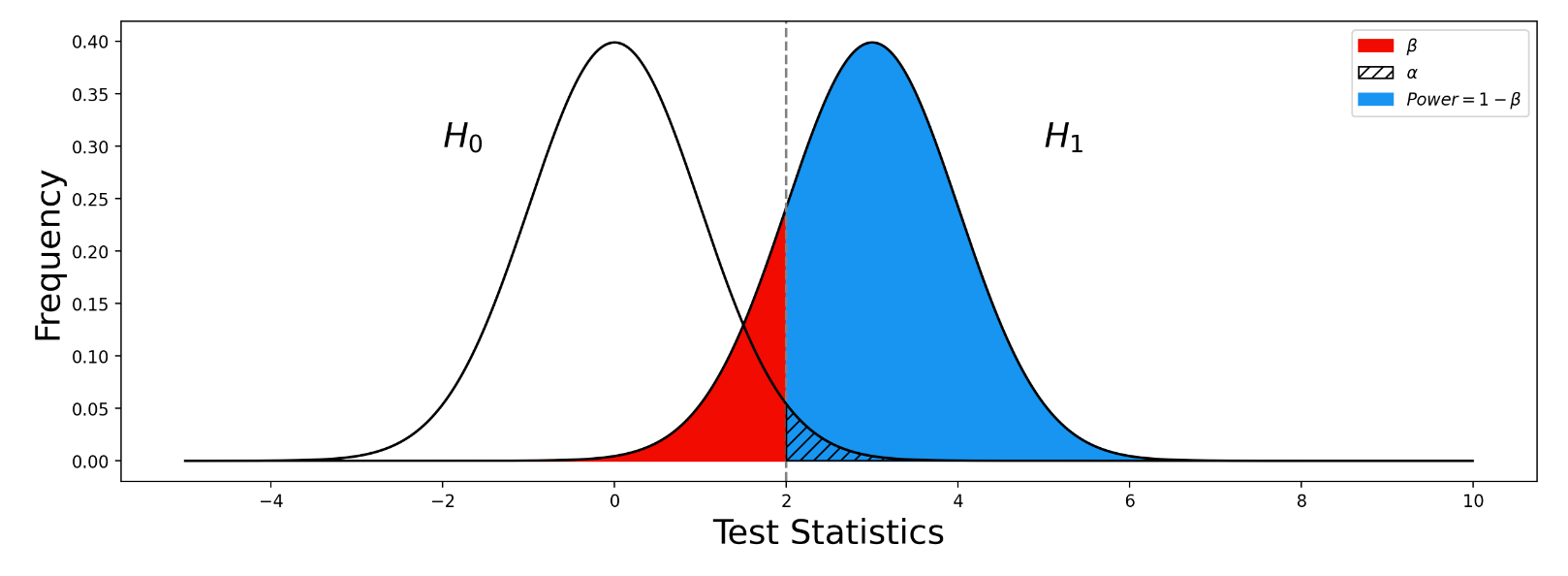
 之间差异的程度。
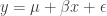


 : 该变异的等位频率(allele frequency)
 分布的非中心参数NCP则为
 :
: 
 : 非中心参数NCP为
 的
的 : 在病例中风险等位的频率 Risk allele frequency in cases
 : 病例的样本量 Number of cases. The total allele count for cases is then
  .
. : 在对照中风险等位的频率 Risk allele frequency in controls
 : 对照的样本量 Number of control. The total allele count for control is then
  .
. , 即风险等位的频率在病例中与对照中是一样的。